Trends

EMSE 4572/6572: Exploratory Data Analysis

John Paul Helveston

October 28, 2026

Quiz 4

Write your name on the quiz!

Rules:

• Work alone; no outside help of any kind is allowed.
• No calculators, no notes, no books, no computers, no phones.

Today’s data

Seen before:

gapminder <- read_csv(file.path('data', 'gapminder.csv'))
milk_production <- read_csv(file.path('data', 'milk_production.csv'))
global_temps <- read_csv(file.path('data', 'nasa_global_temps.csv'))
internet_region <- read_csv(file.path('data', 'internet_users_region.csv'))
hotdogs <- read_csv(file.path('data', 'hot_dog_winners.csv'))
internet_country <- read_csv(file.path('data', 'internet_users_country.csv'))

New datasets:

us_covid <- read_csv(file.path('data', 'us_covid.csv'))
us_diseases <- read_csv(file.path('data', 'us_contagious_diseases.csv'))

New packages:

install.packages('viridis')
install.packages('gganimate')
install.packages('magick')

Week 10: Trends

1. Single Variables

2. Animations

3. Multiple Variables

Week 10: Trends

1. Single Variables

2. Animations

3. Multiple Variables

Points

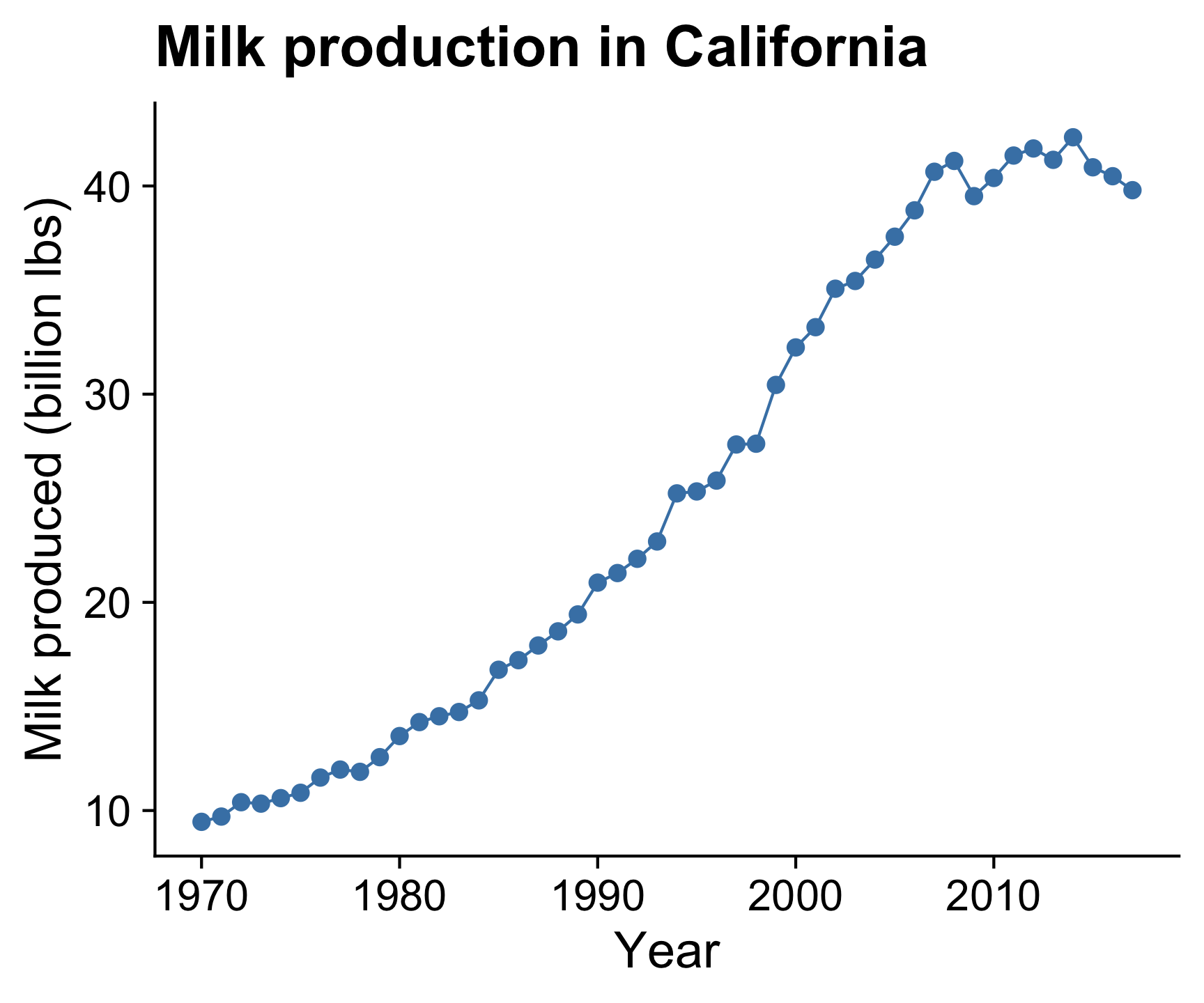
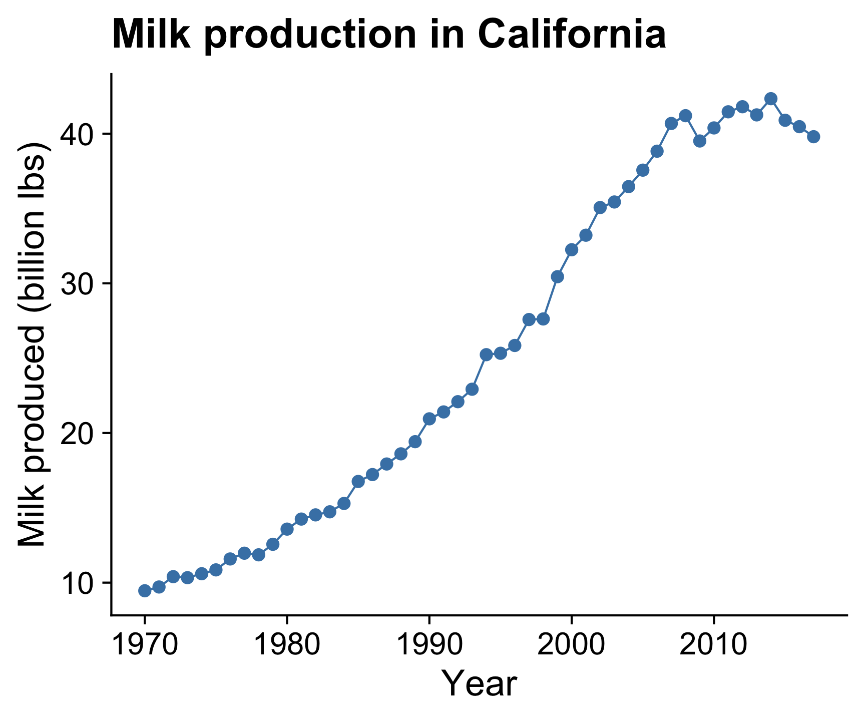
Plotting the data points is a good starting point for viewing trends

Points + line

Adding lines between the points helps
see the overall trend

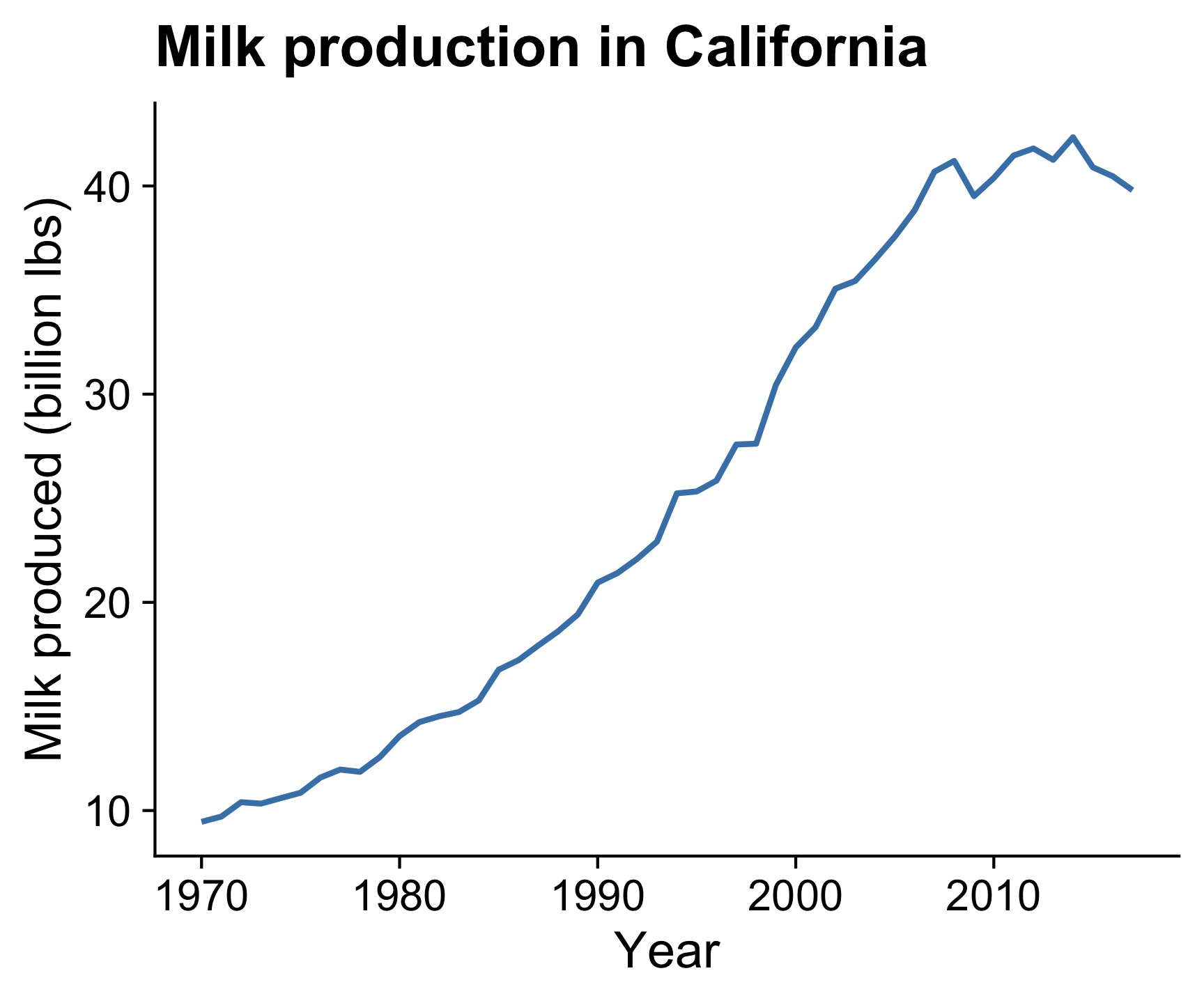
Line

Omitting the points emphasizes the overall trend

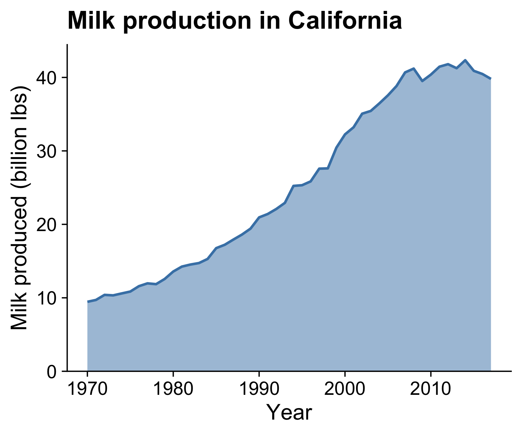
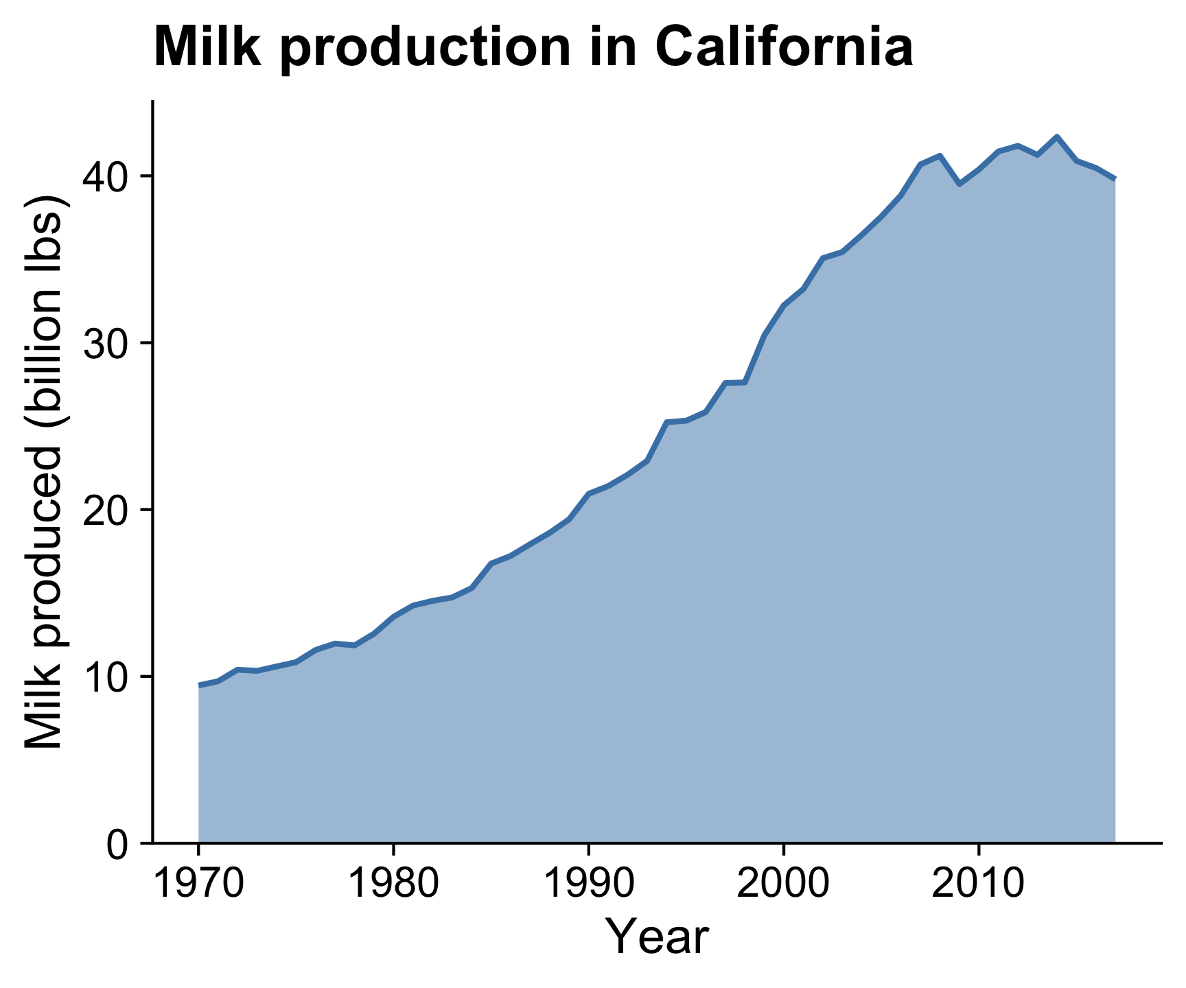
Line + area

Filling area below line emphasizes cumulative over time

(y-axis should start at 0)

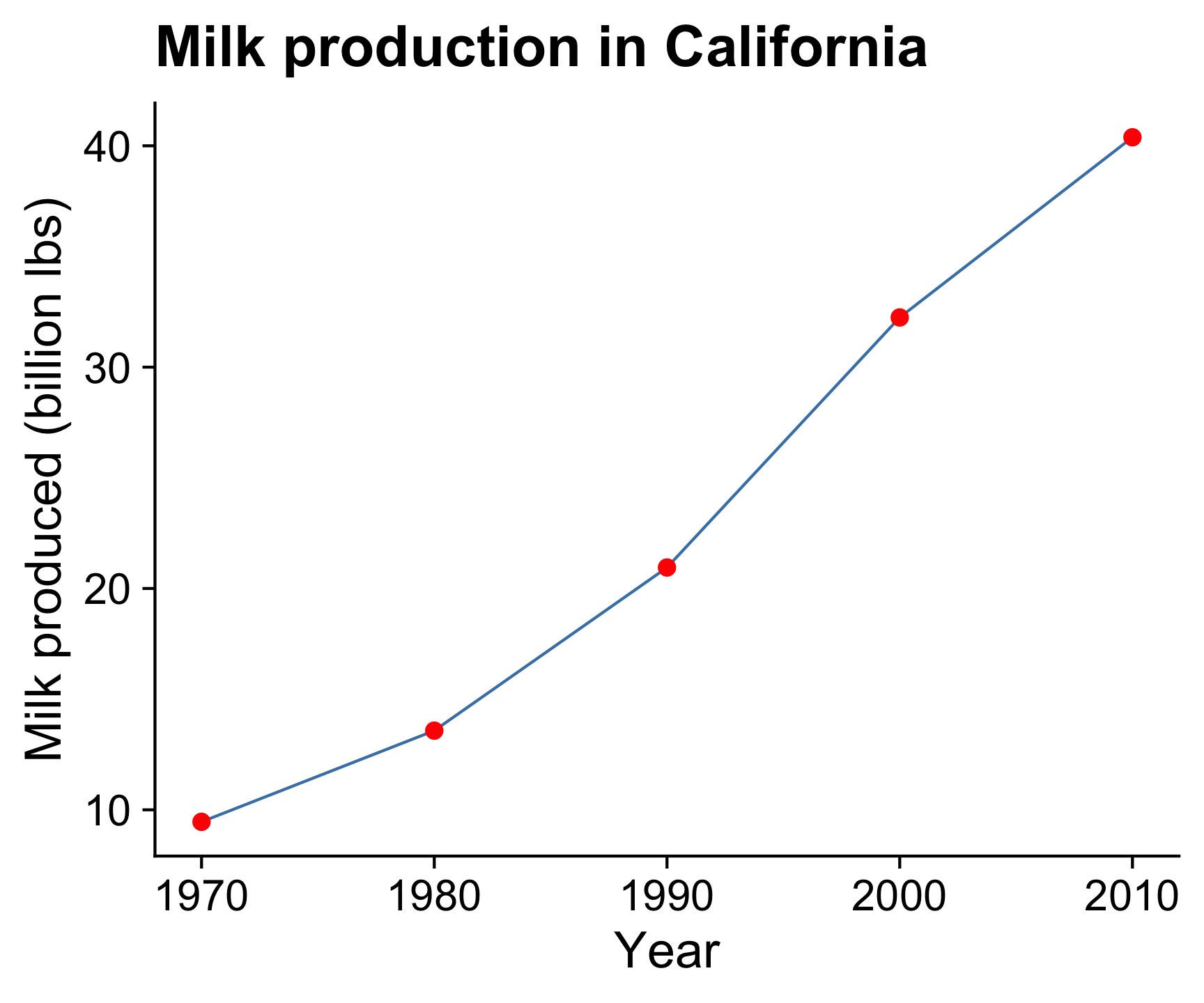
If points are too sparse, a line can be misleading

Smoothed line

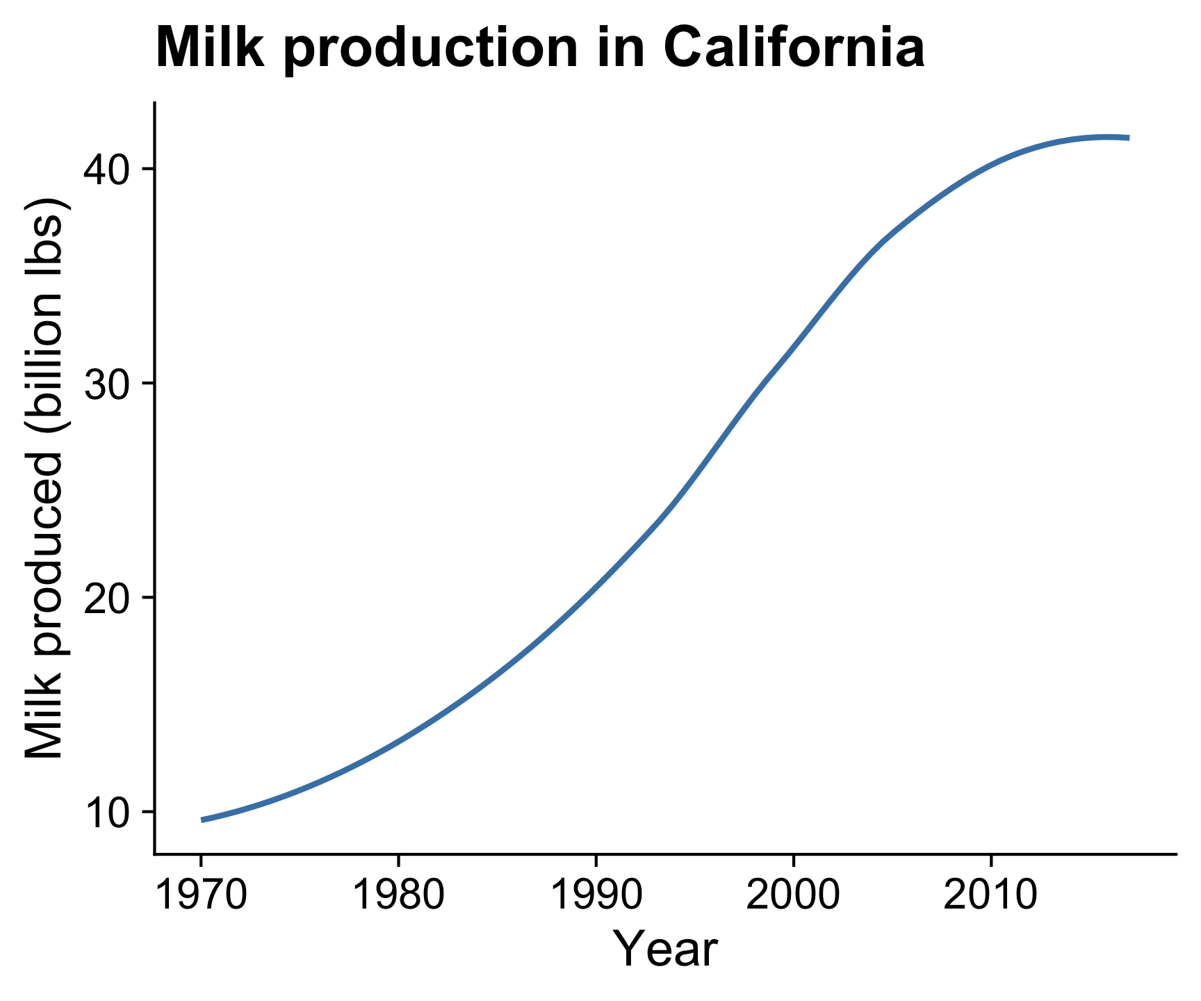
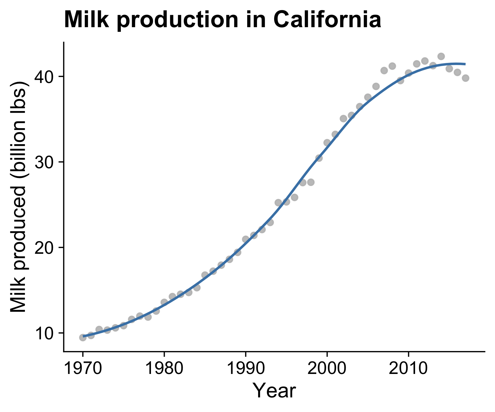
Adding a “smoothed” line shows a modeled representation of the overall trend

Smoothed line + points

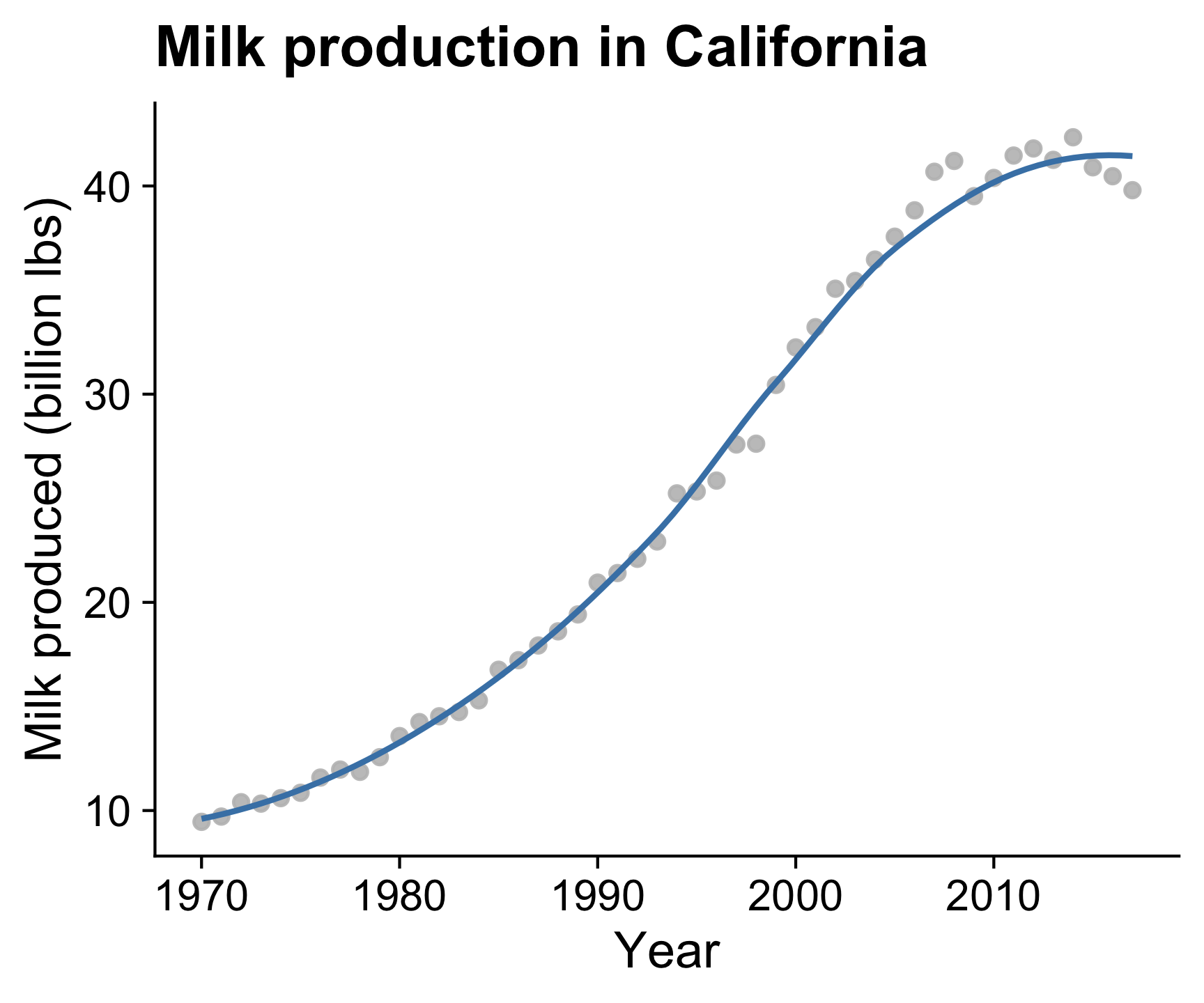
Putting the smoothed line over the data points helps show whether outliers are driving the trend line

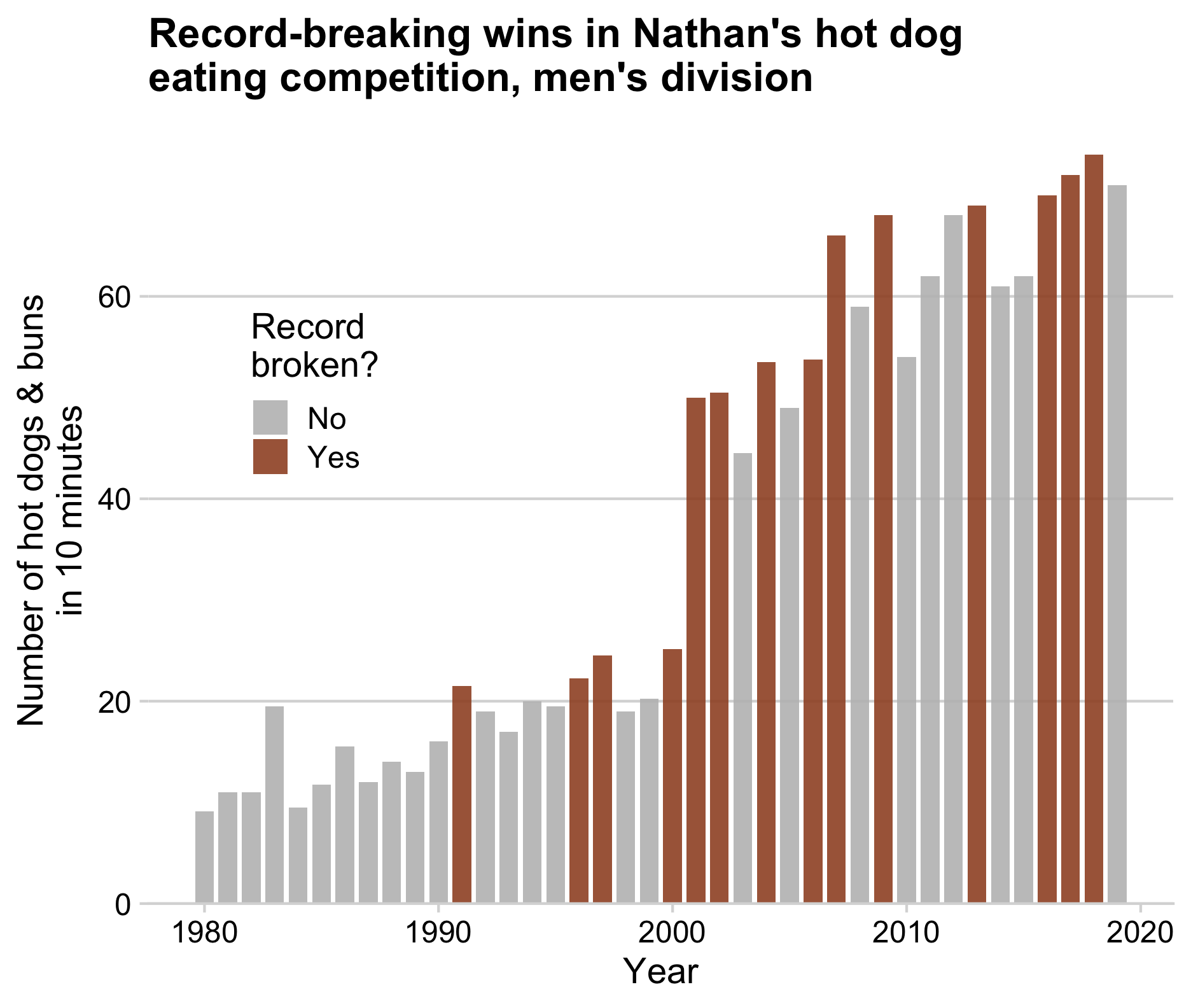
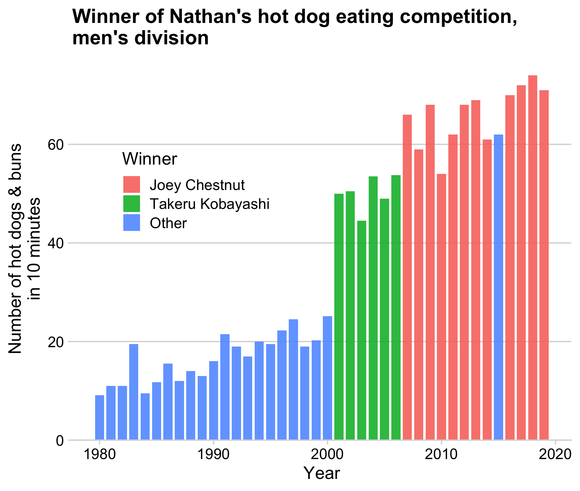
Bars are useful when emphasizing the data points
rather than the slope between them

How to: Points + line

Be sure to draw the line first,
then overlay the points

ggplot(milk_ca, aes(x = year, y = milk_produced)) +
    geom_line(color = 'steelblue', size = 0.5) +
    geom_point(color = 'steelblue', size = 2) +
    theme_half_open(font_size = 18) +
    labs(
        x = 'Year',
        y = 'Milk produced (billion lbs)',
        title = 'Milk production in California'
    )

How to: Line + area

Likewise, draw the area first then overlay the line

ggplot(milk_ca, aes(x = year, y = milk_produced)) +
    geom_area(fill = 'steelblue', alpha = 0.5) +
    geom_line(color = 'steelblue', size = 1) +
    scale_y_continuous(
        expand = expansion(mult = c(0, 0.05))
    ) +
    theme_half_open(font_size = 18) +
    labs(
        x = 'Year',
        y = 'Milk produced (billion lbs)',
        title = 'Milk production in California'
    )

How to: Smoothed line + points

Use alpha to make points slightly transparent

ggplot(milk_ca, aes(x = year, y = milk_produced)) +
  geom_point(color = 'grey', size = 2, alpha = 0.9) +
  geom_smooth(color = 'steelblue', size = 1, se = FALSE) +
  theme_half_open(font_size = 18) +
  labs(
    x = 'Year',
    y = 'Milk produced (billion lbs)',
    title = 'Milk production in California'
  )

Your turn

Use the global_temps data frame to explore ways to visualize the change in average global temperatures.

Consider using:

• points
• lines
• areas
• smoothed lines

global_temps <- read_csv(file.path(
  'data',
  'nasa_global_temps.csv'
))

head(global_temps)

#> # A tibble: 6 × 3
#>    year meanTemp smoothTemp
#>   <dbl>    <dbl>      <dbl>
#> 1  1880    -0.15      -0.08
#> 2  1881    -0.07      -0.12
#> 3  1882    -0.1       -0.15
#> 4  1883    -0.16      -0.19
#> 5  1884    -0.27      -0.23
#> 6  1885    -0.32      -0.25

Week 10: Trends

1. Single Variables

2. Animations

3. Multiple Variables

Animation adds emphasis to the change over time

…plus it’s fun!

Static chart

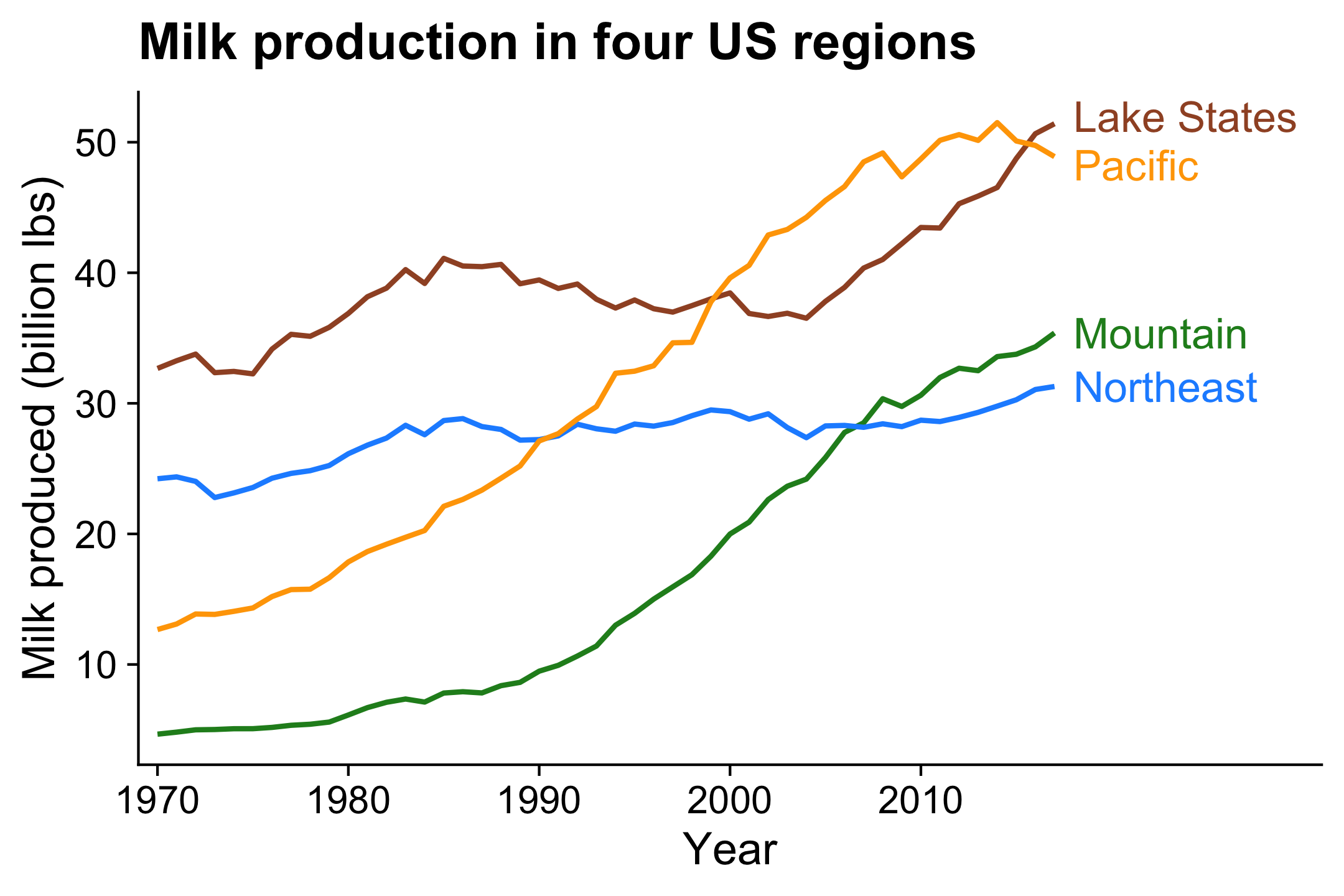
Animated chart

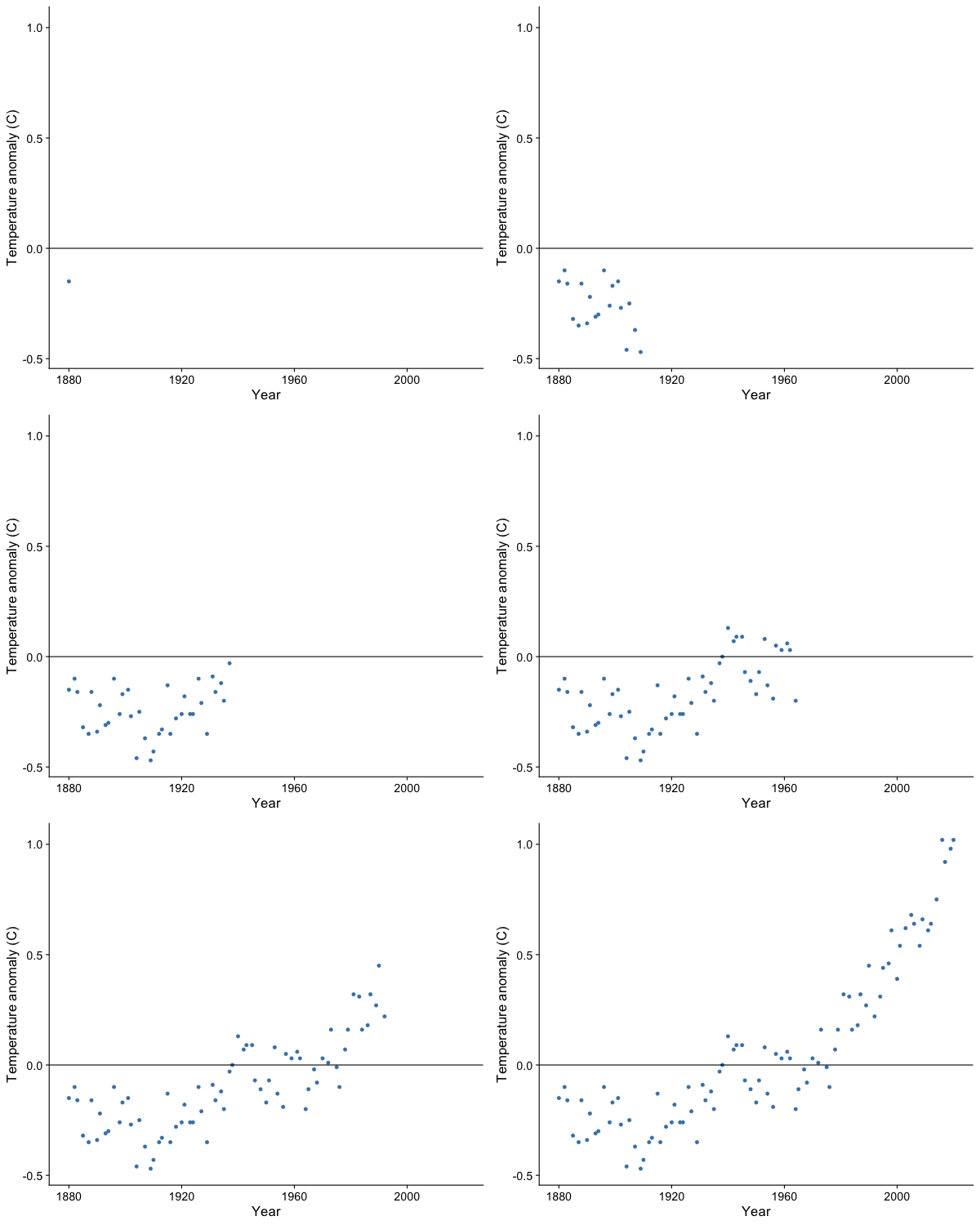
Animation is particularly helpful for the time dimension

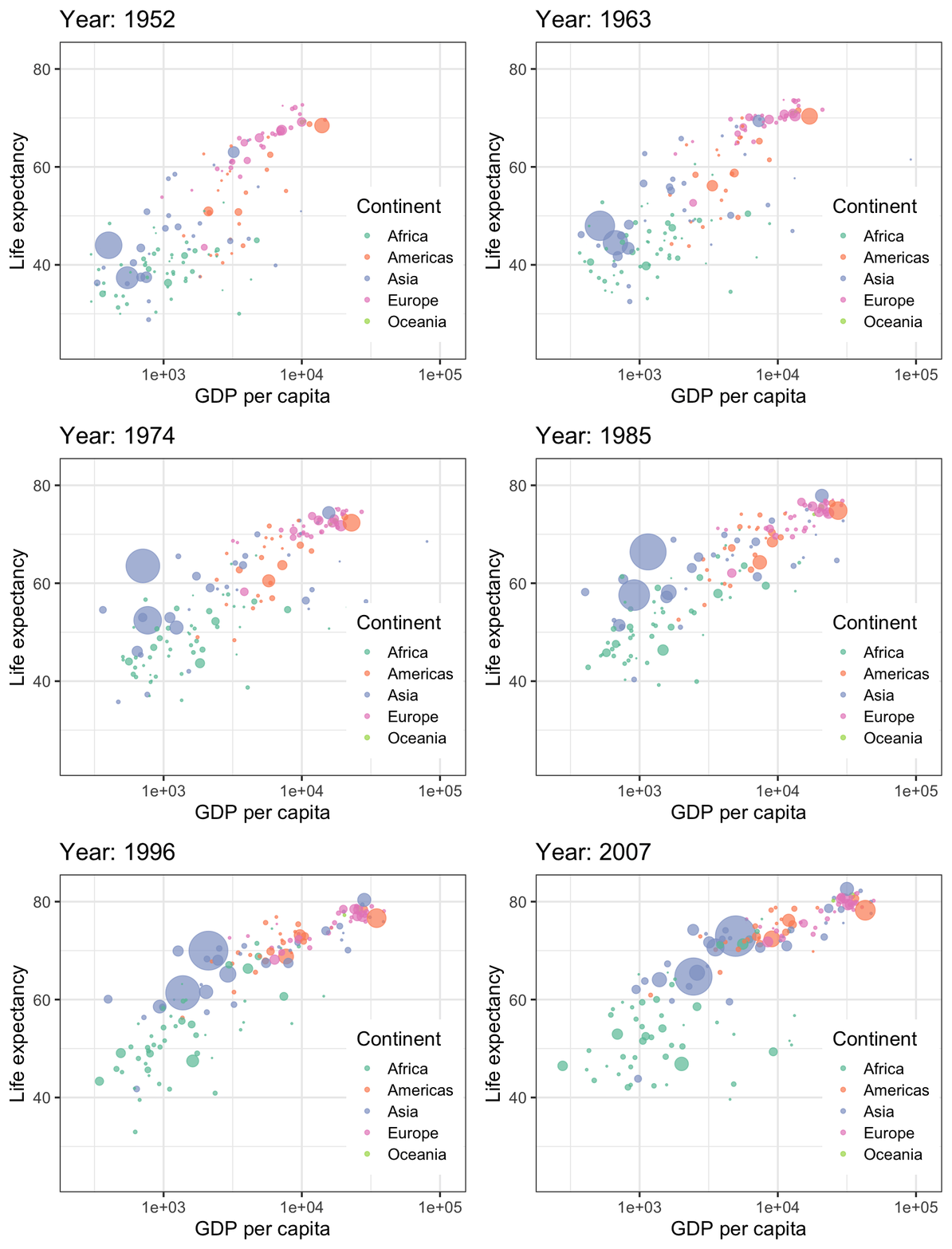
“Gapminder” visualization by Hans Rosling

Animation is particularly helpful for the time dimension

Source: https://www.climate-lab-book.ac.uk/spirals/

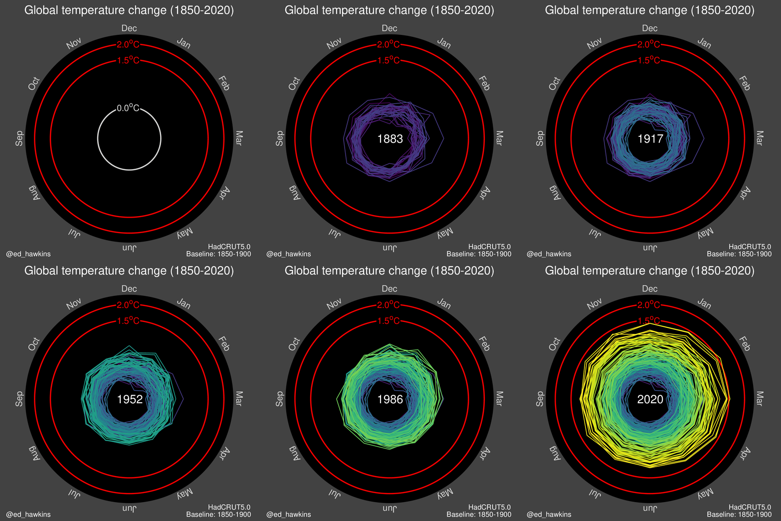
Animation is particularly helpful for the time dimension

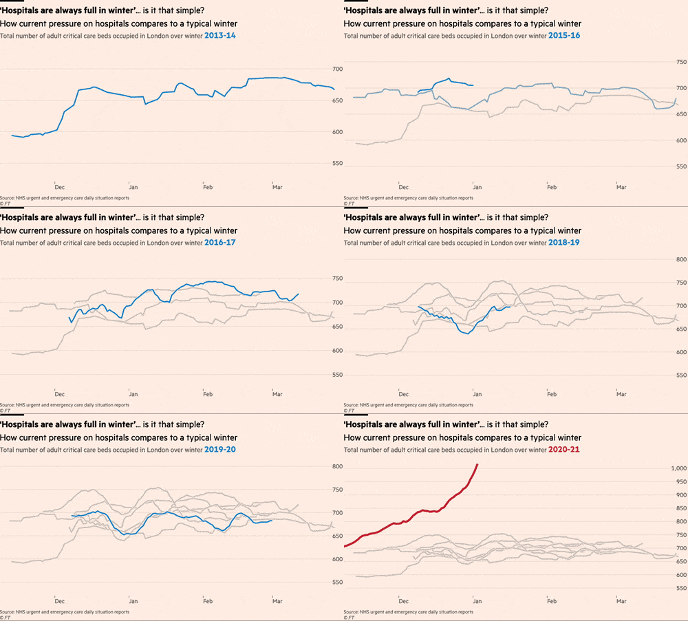
Financial Times comparison of Flu seasons to COVID-19

Animation is particularly helpful for the time dimension

“Bar chart race” of top 10 milk producing states

How to: Animate a line plot

Make a static plot w/labels for each year

milk_region_anim_plot <- milk_region %>%
  ggplot(aes(x = year, y = milk_produced, color = region)) +
  geom_line(size = 1) +
  geom_point(size = 2) +
  geom_text_repel(
    aes(label = region),
    hjust = 0,
    nudge_x = 1,
    direction = "y",
    size = 6,
    segment.color = NA
  ) +
  scale_x_continuous(
    breaks = seq(1970, 2010, 10),
    expand = expansion(add = c(1, 13))
  ) +
  scale_color_manual(
    values = c('sienna', 'forestgreen', 'dodgerblue', 'orange')
  ) +
  theme_half_open(font_size = 18) +
  theme(legend.position = 'none') +
  labs(
    x = 'Year',
    y = 'Milk produced (billion lbs)',
    title = 'Milk production in four US regions'
  )

milk_region_anim_plot

milk_region_anim_plot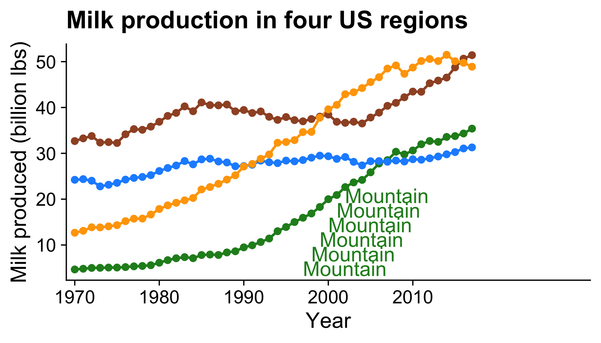

How to: Animate a line plot

Now animate it

Note the pause at the end!

library(gganimate)

milk_region_anim <- milk_region_anim_plot +
    transition_reveal(year)

# Render the animation
animate(
    milk_region_anim,
    end_pause = 15,
    duration = 10,
    width = 1100,
    height = 650,
    res = 150,
    renderer = magick_renderer()
)

# Save last animation
anim_save(file.path(
    'figs',
    'milk_region_animation.gif'
))

How to: Change label based on year

First make a static plot

gapminder_anim_plot <- ggplot(
  gapminder,
  aes(x = gdpPercap, y = lifeExp, size = pop, color = continent)
) +
  geom_point(alpha = 0.7) +
  scale_size_area(guide = FALSE, max_size = 15) +
  scale_color_brewer(palette = 'Set2') +
  scale_x_log10() +
  theme_bw(base_size = 18) +
  theme(legend.position = c(0.85, 0.3)) +
  labs(x = 'GDP per capita', y = 'Life expectancy', color = 'Continent')

gapminder_anim_plot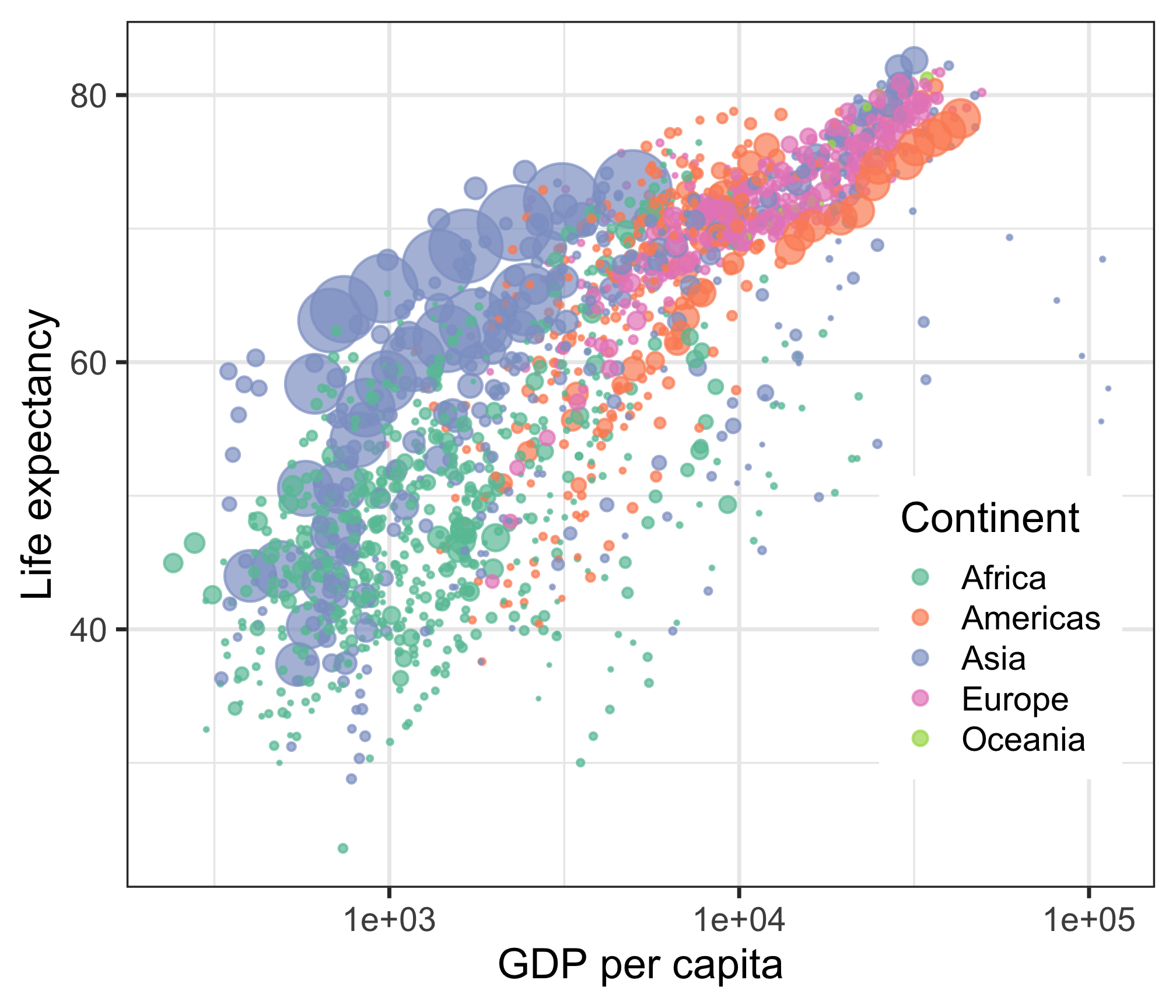

How to: Change label based on year

Now animate it

Note: Year must be an integer!

gapminder_anim <- gapminder_anim_plot +
  transition_time(year) +
  labs(title = "Year: {frame_time}")

# Render the animation
animate(
  gapminder_anim,
  end_pause = 10,
  width = 800,
  height = 600,
  res = 150,
  renderer = magick_renderer()
)

milk_race_anim <- milk_production %>%
  group_by(year) %>%
  mutate(
    rank = rank(-milk_produced),
    Value_rel = milk_produced / milk_produced[rank == 1],
    Value_lbl = paste0(' ', round(milk_produced))
  ) %>%
  group_by(state) %>%
  filter(rank <= 10) %>%
  ungroup() %>%
  mutate(year = as.integer(year)) %>%
  ggplot(aes(x = rank, group = state, fill = region, color = region)) +
  geom_tile(
    aes(y = milk_produced / 2, height = milk_produced),
    width = 0.9,
    alpha = 0.8,
    color = NA
  ) +
  geom_text(aes(y = 0, label = paste(state, " ")), vjust = 0.2, hjust = 1) +
  geom_text(aes(y = milk_produced, label = Value_lbl), hjust = 0) +
  coord_flip(clip = 'off', expand = FALSE) +
  scale_y_continuous(labels = scales::comma) +
  scale_fill_viridis(discrete = TRUE) +
  scale_color_viridis(discrete = TRUE) +
  scale_x_reverse() +
  guides(color = FALSE) +
  theme_minimal_vgrid() +
  transition_time(year) +
  view_follow(fixed_x = TRUE) +
  theme(
    axis.line = element_blank(),
    axis.text = element_blank(),
    axis.ticks = element_blank(),
    axis.title = element_blank(),
    legend.position = c(0.7, 0.3),
    legend.background = element_rect(fill = 'white'),
    plot.title = element_text(
      size = 22,
      hjust = 0.5,
      face = 'bold',
      colour = 'grey',
      vjust = -1
    ),
    plot.subtitle = element_text(
      size = 18,
      hjust = 0.5,
      face = 'italic',
      color = 'grey'
    ),
    plot.caption = element_text(
      size = 8,
      hjust = 0.5,
      face = 'italic',
      color = 'grey'
    ),
    plot.margin = margin(0.5, 2, 0.5, 3, 'cm')
  ) +
  labs(
    title = 'Year : {frame_time}',
    subtitle = 'Top 10 states by milk produced',
    fill = 'Region',
    caption = 'Milk produced (billions lbs)'
  )

Making a bar chart race
(tutorial here)

animate(
        milk_race_anim,
        duration = 17,
        end_pause = 15,
        width = 800,
        height = 700,
        res = 150,
        renderer = magick_renderer()
)

Resources

More animation options:

• More on gapminder + line charts
• Customizing the animation

Your turn

Use the global_temps data frame to explore ways to animate the change in average global temperatures.

Consider using:

• points
• lines
• areas

Break!

Stand up, Move around, Stretch!

Week 10: Trends

1. Single Variables

2. Animations

3. Multiple Variables

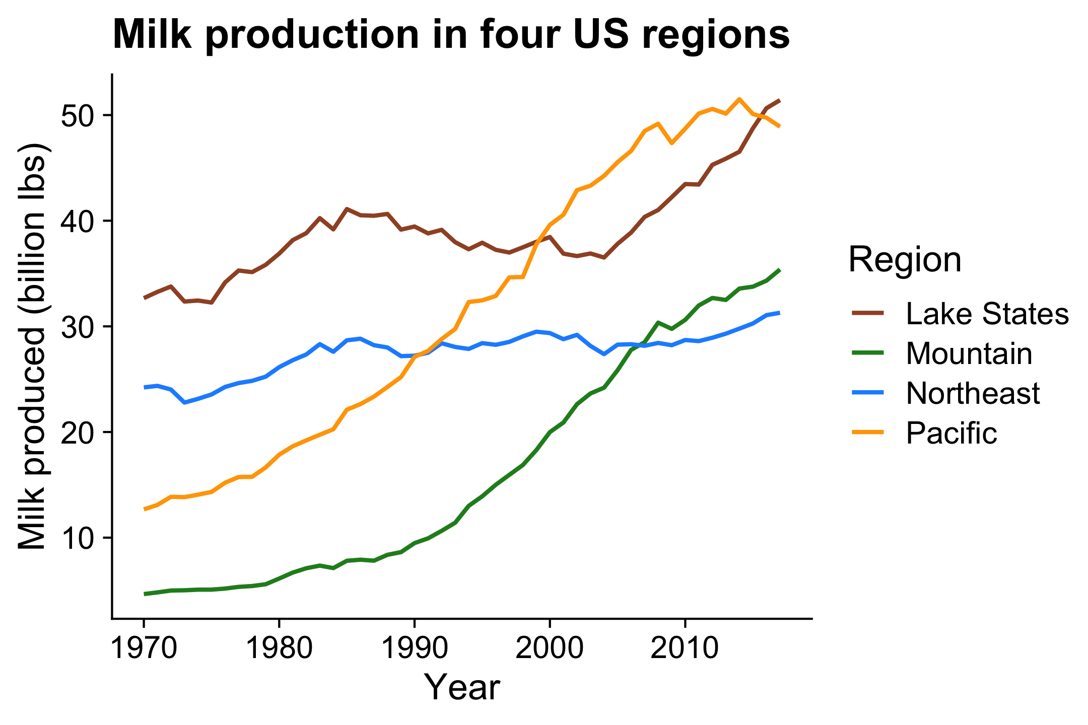
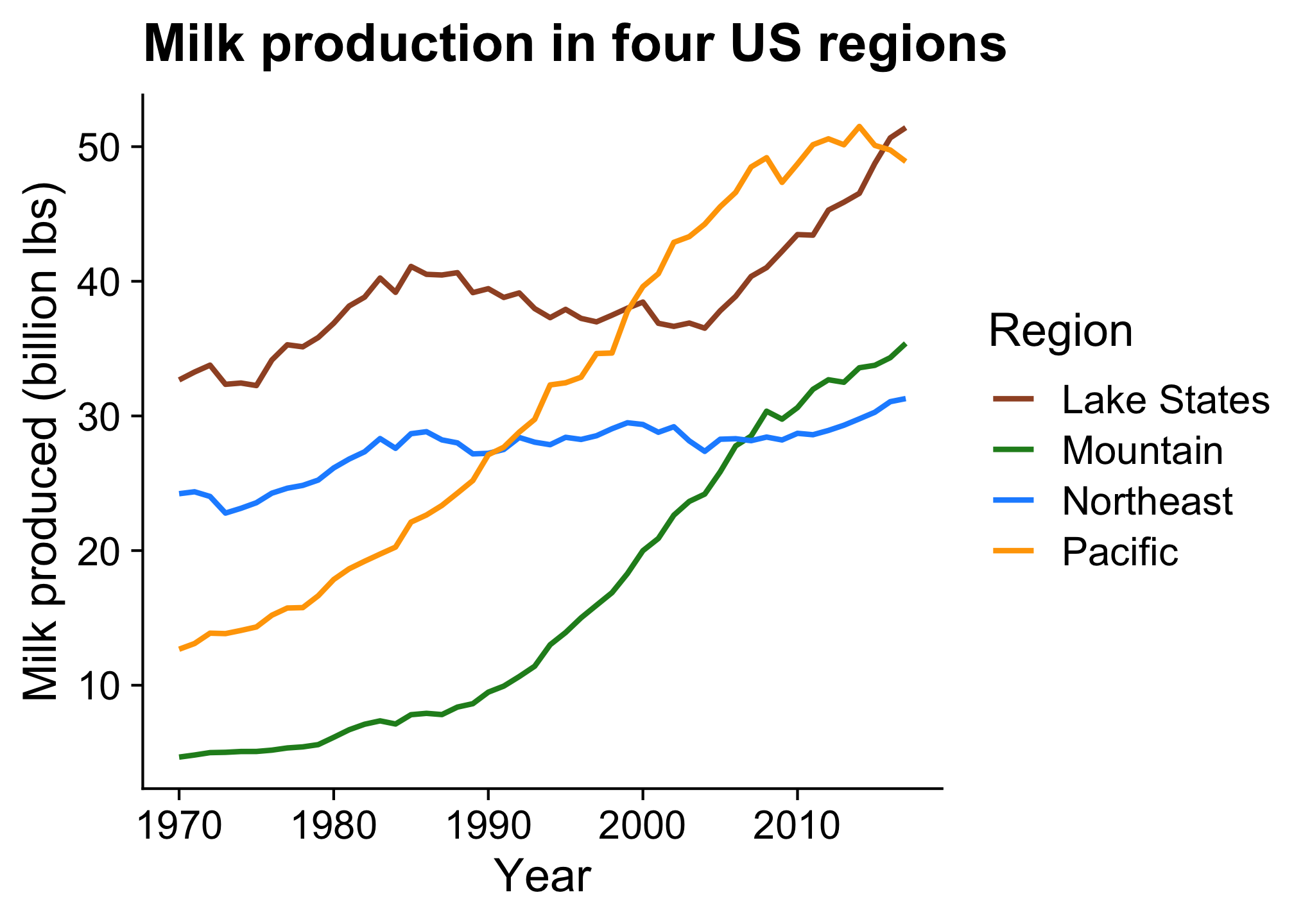
With multiple categories,
points & lines can get messy

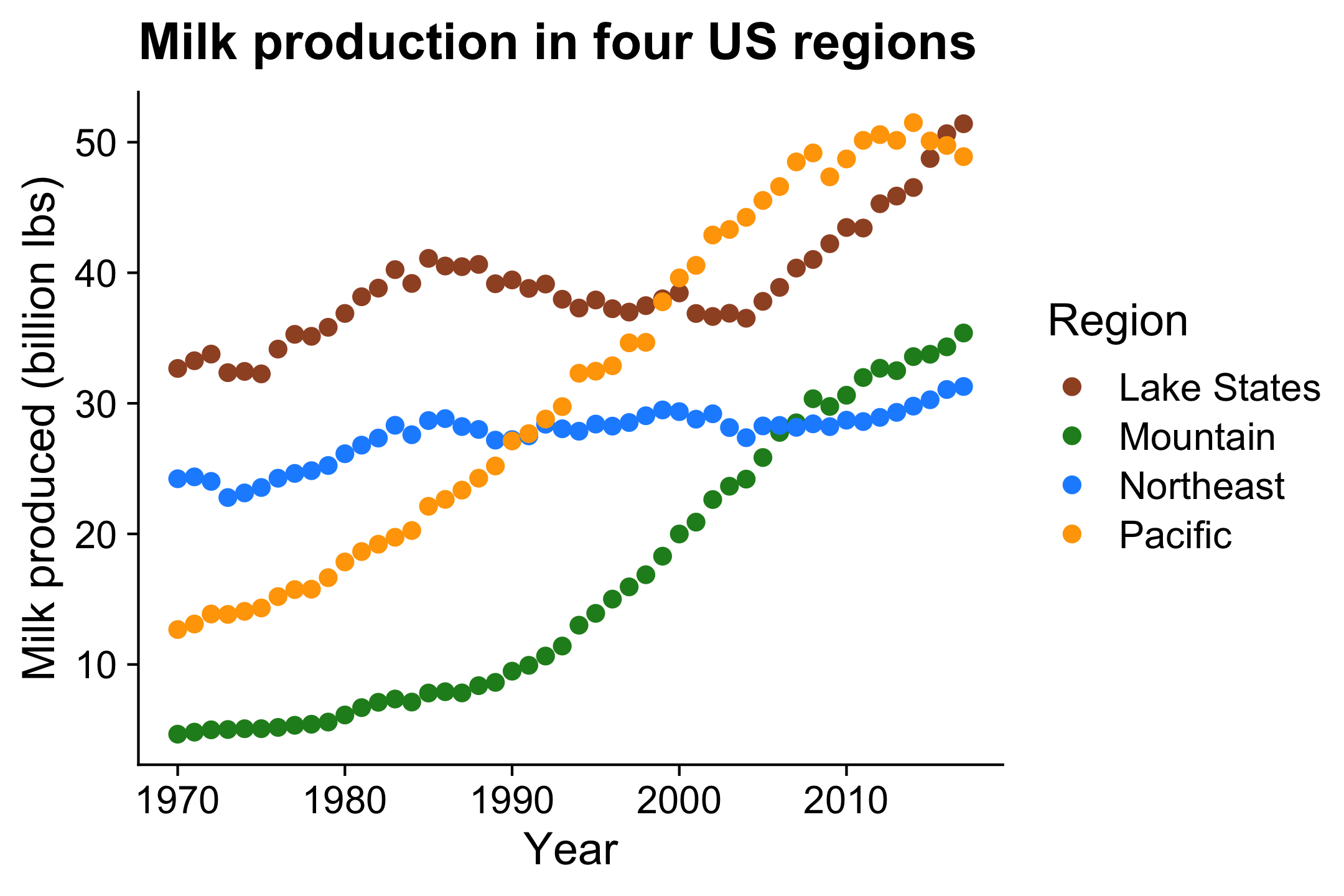
Better: Lines alone makes distinguishing trends easier

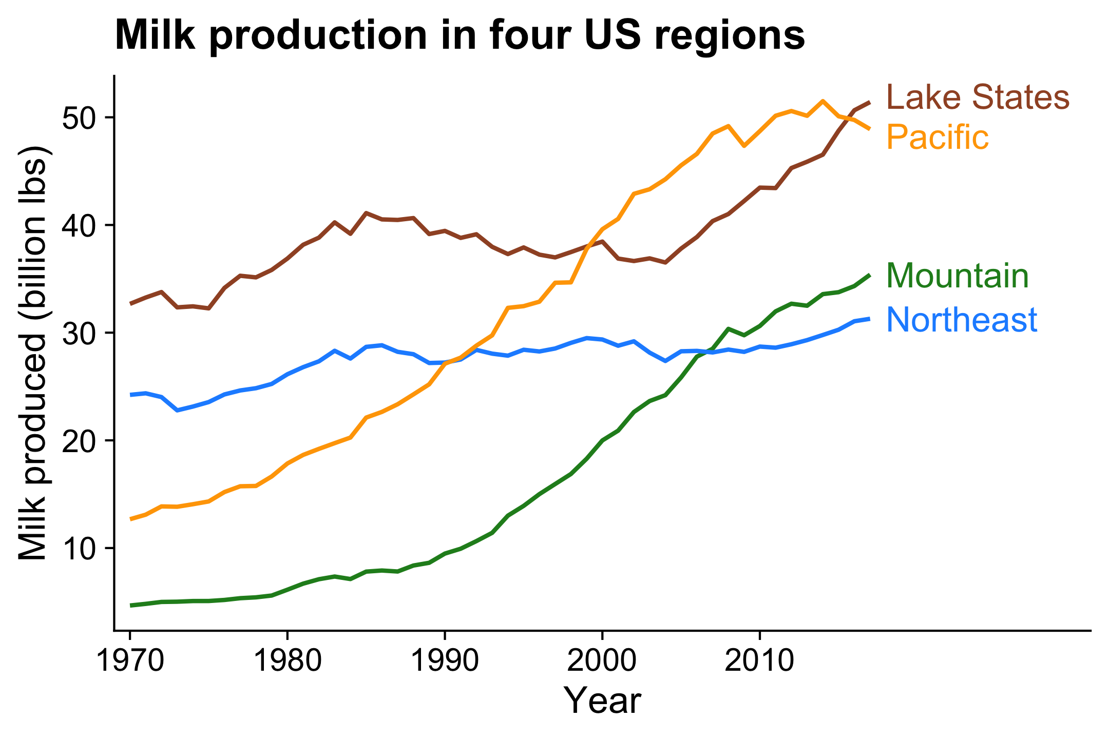
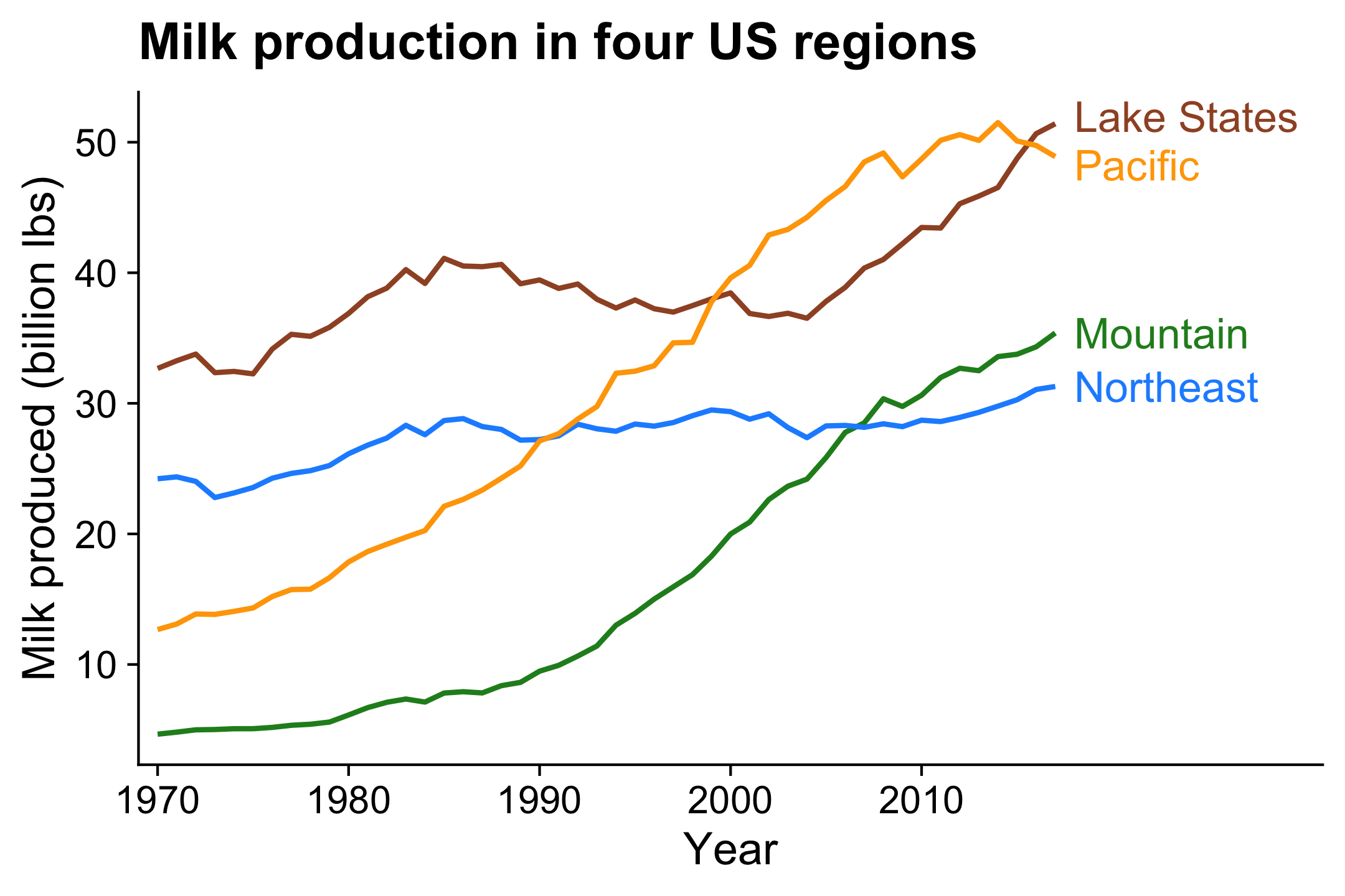
Even better: Directly label
lines to remove legend

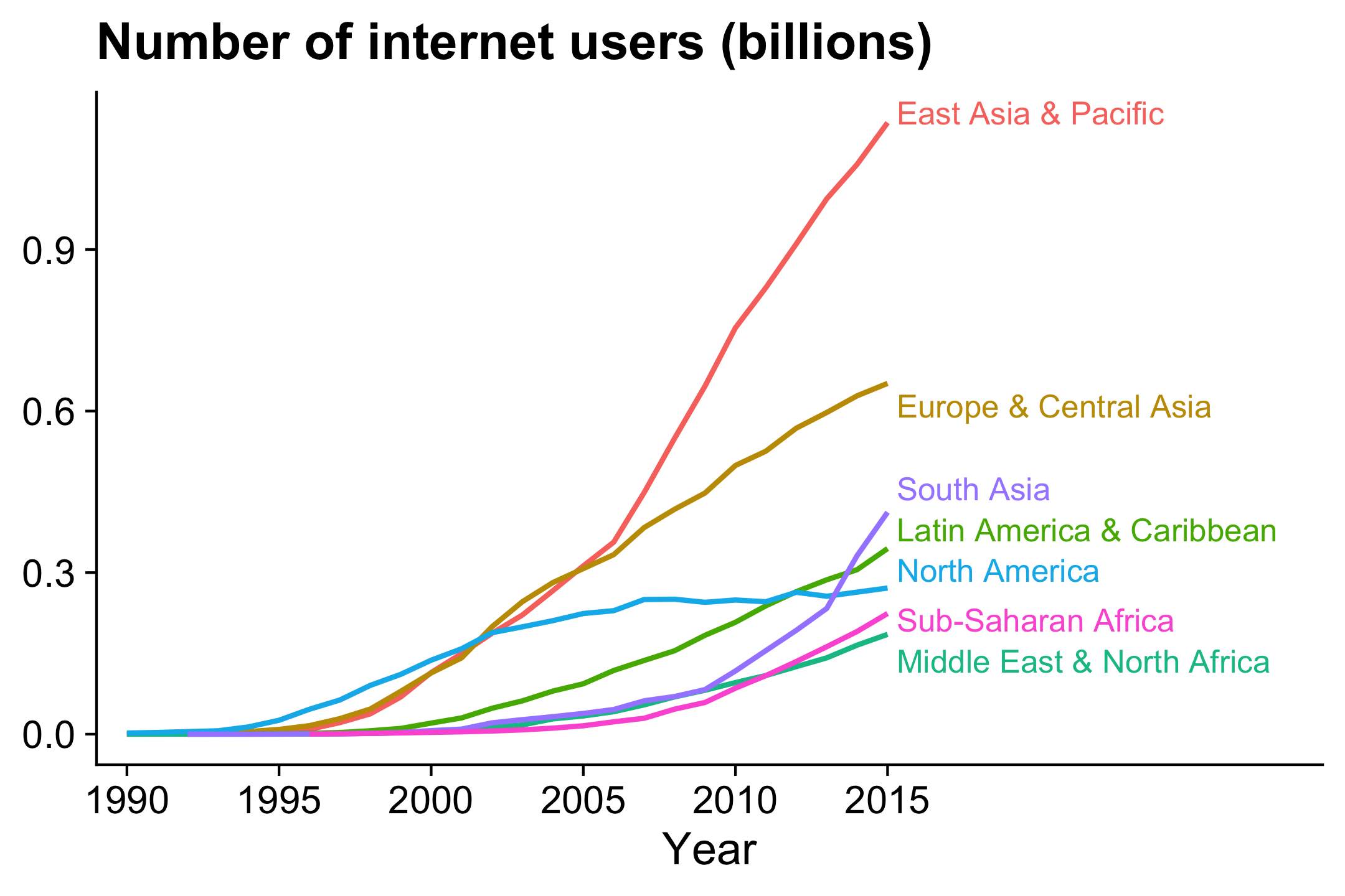
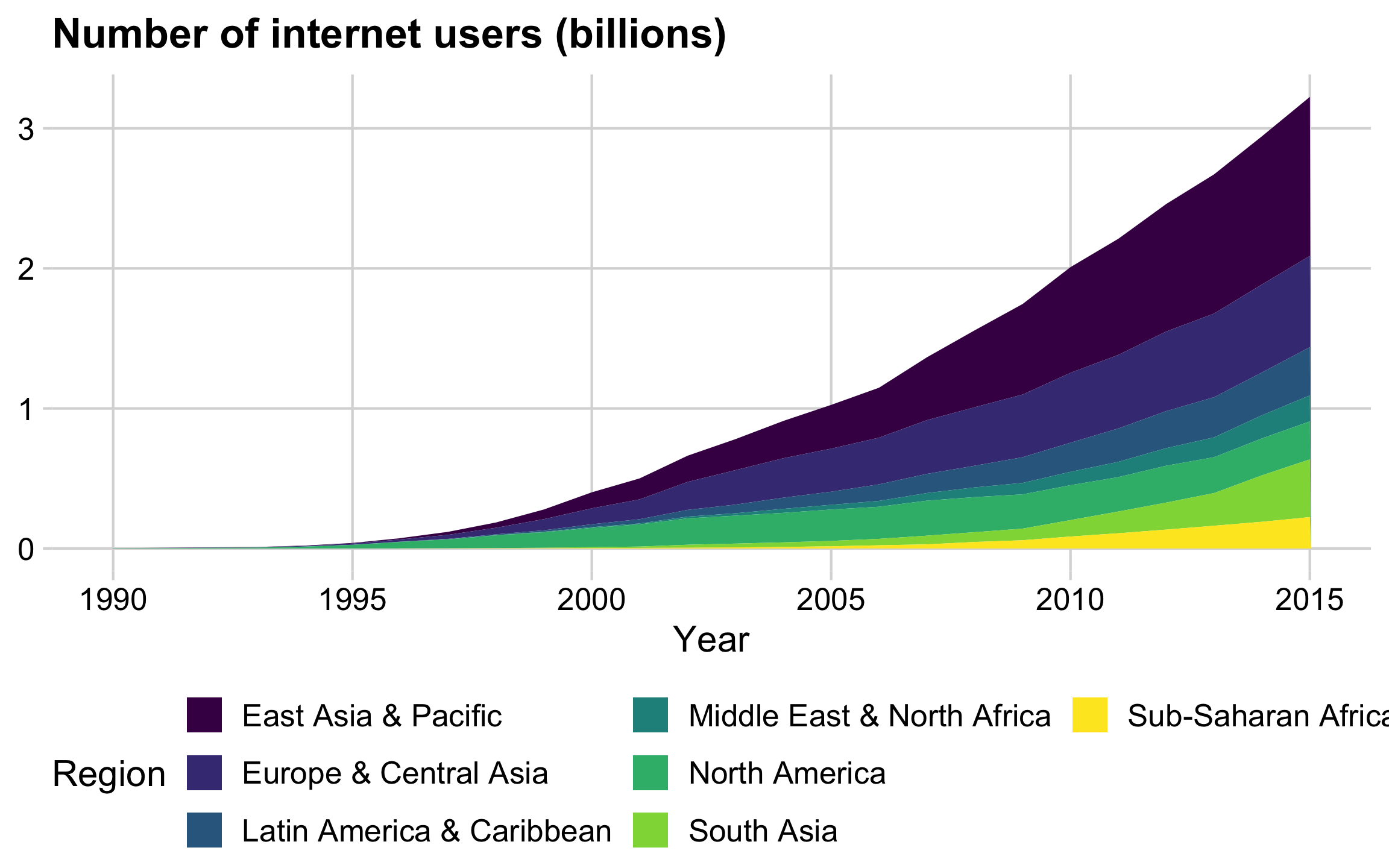
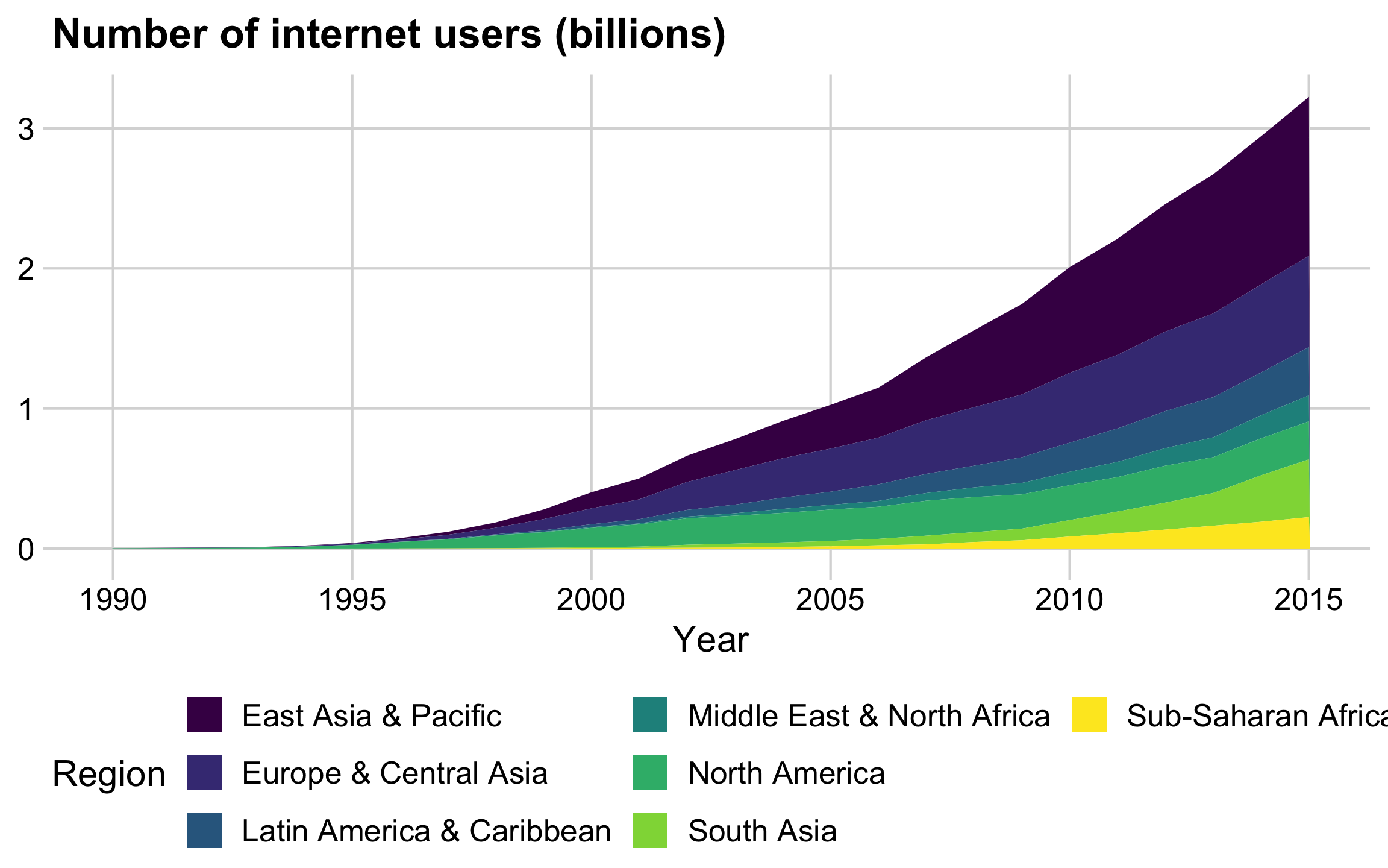
If goal is to communicate the overall / total trend,
consider a stacked area chart

Highlights regional trends

Highlights overall / total trend

If you have lots of categories:
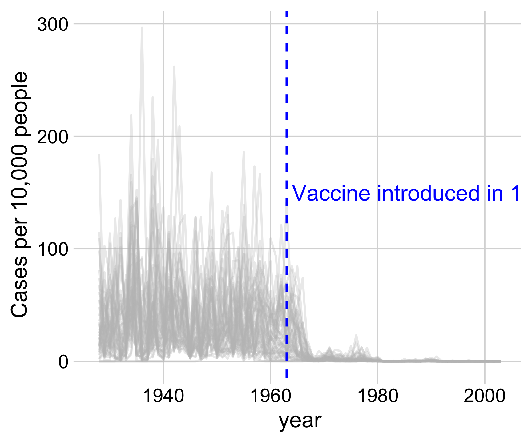
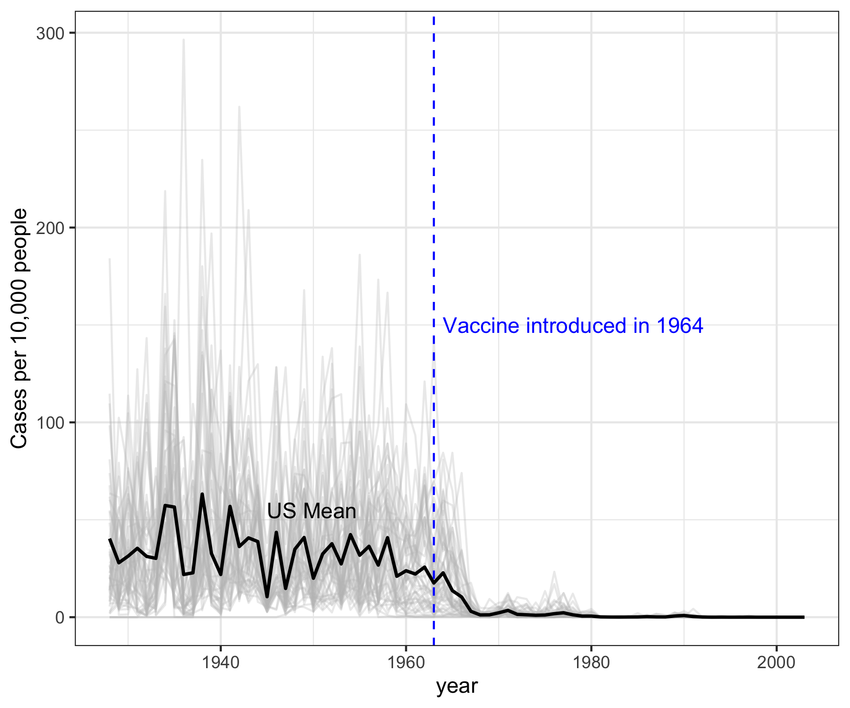
1) Plot all the data with the average highlighted

Measles in California

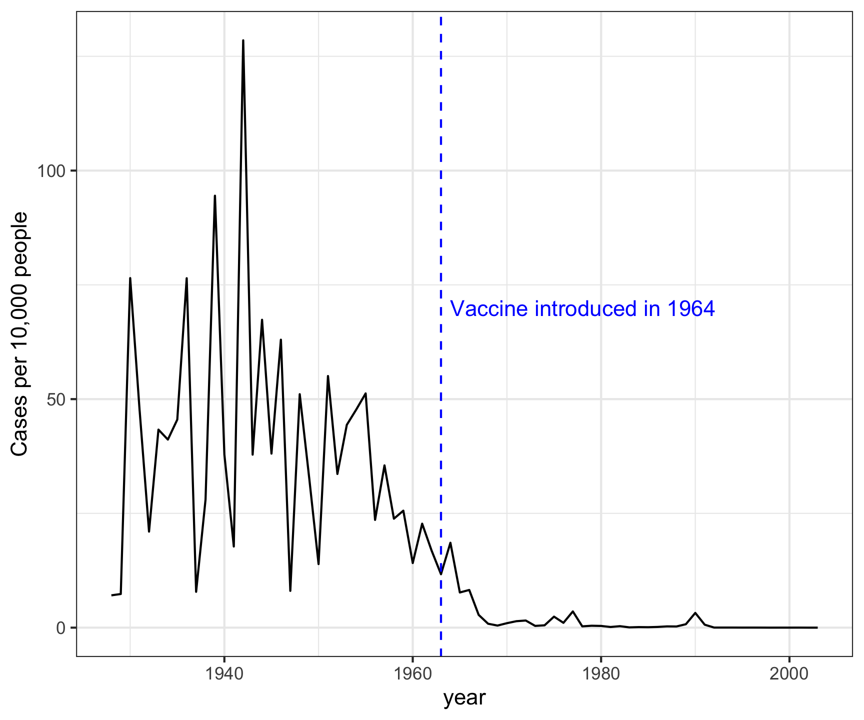
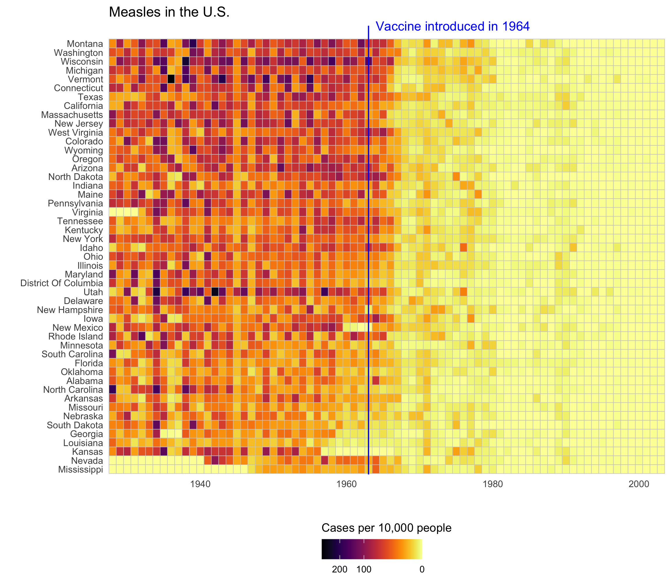
Measles in all 50 states

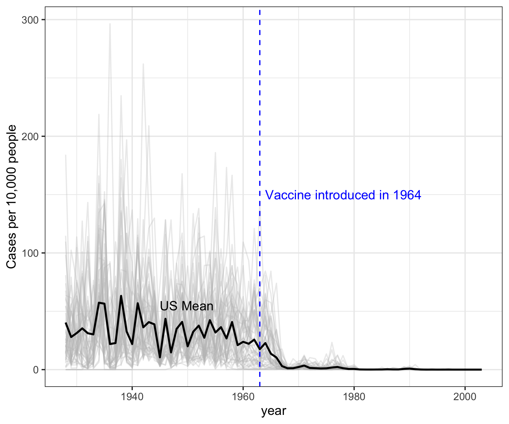
If you have lots of categories:
1) Plot all the data with the average highlighted
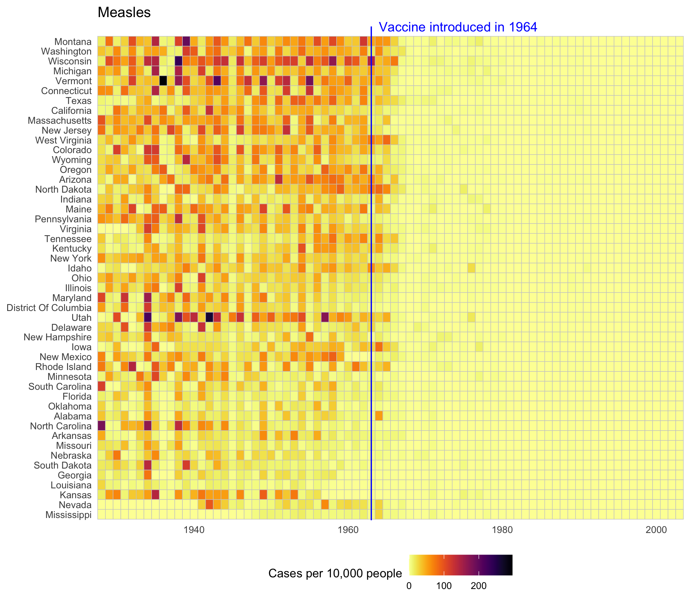
2) Plot all the data with a heat map

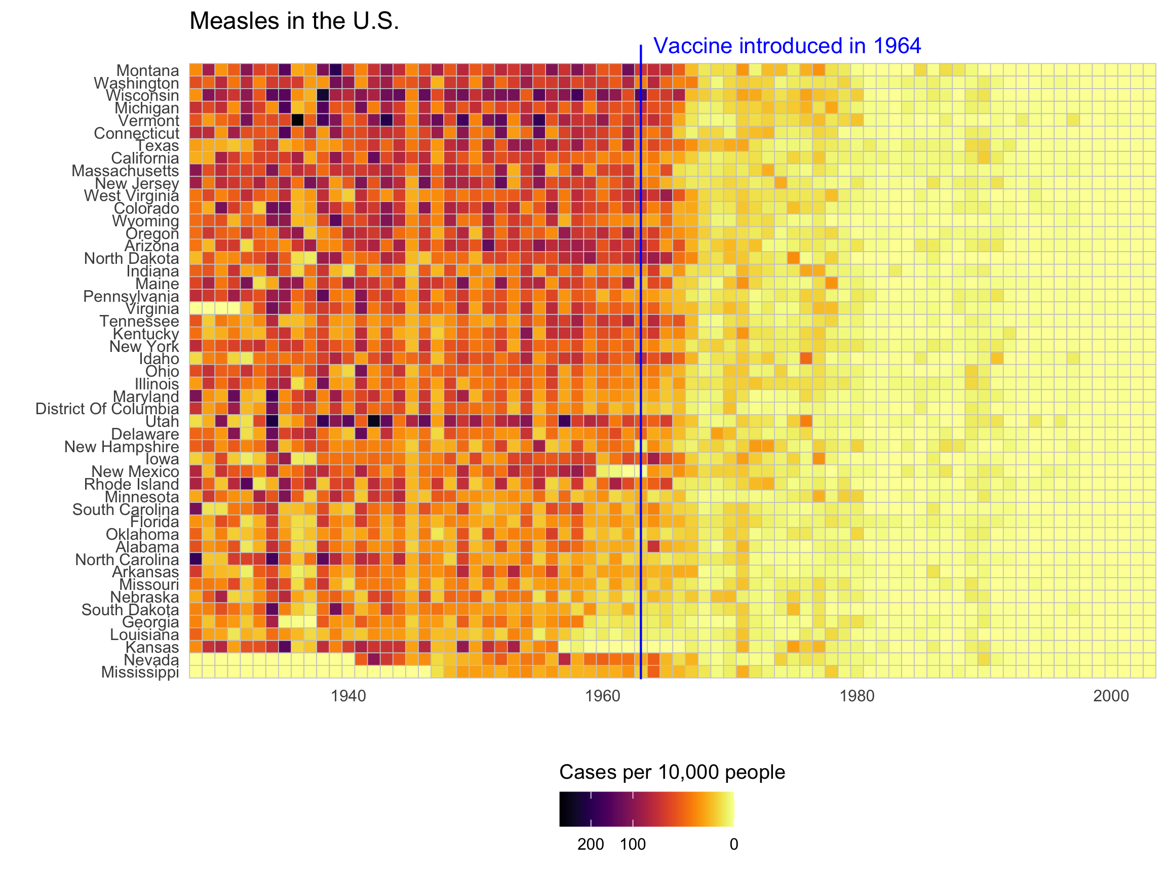
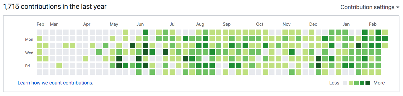
Heatmaps are great for multiple divisions of time

My activity on Github:

Check out this heat map on Traffic fatalities

Make the basic line chart first

# Format the data
milk_region <- milk_production %>%
  filter(
    region %in%
      c('Pacific', 'Northeast', 'Lake States', 'Mountain')
  ) %>%
  group_by(year, region) %>%
  summarise(milk_produced = sum(milk_produced)) %>%
  ungroup()

# Make the line chart
ggplot(
  milk_region,
  aes(x = year, y = milk_produced, color = region)
) +
  geom_line(size = 1) +
  scale_color_manual(
    values = c('sienna', 'forestgreen', 'dodgerblue', 'orange')
  ) +
  theme_half_open(font_size = 18) +
  labs(
    x = 'Year',
    y = 'Milk produced (billion lbs)',
    color = 'Region',
    title = 'Milk production in four US regions'
  )

How to:
Directly label lines

# Format the data
milk_region <- milk_production %>%
  filter(
    region %in%
      c('Pacific', 'Northeast', 'Lake States', 'Mountain')
  ) %>%
  group_by(year, region) %>%
  summarise(milk_produced = sum(milk_produced)) %>%
  ungroup()

# Make the line plot
ggplot(milk_region, aes(x = year, y = milk_produced, color = region)) +
  geom_line(size = 1) +
  # Add labels
  geom_text_repel(
    data = milk_region %>% filter(year == max(year)),
    aes(label = region),
    hjust = 0,
    nudge_x = 1,
    direction = "y",
    size = 6,
    segment.color = NA
  ) +
  # Create space for labels on right side
  scale_x_continuous(
    breaks = seq(1970, 2010, 10),
    expand = expansion(add = c(1, 13))
  ) +
  scale_color_manual(
    values = c('sienna', 'forestgreen', 'dodgerblue', 'orange')
  ) +
  theme_half_open(font_size = 18) +
  # Remove legend
  theme(legend.position = 'none') +
  labs(
    x = 'Year',
    y = 'Milk produced (billion lbs)',
    title = 'Milk production in four US regions'
  )

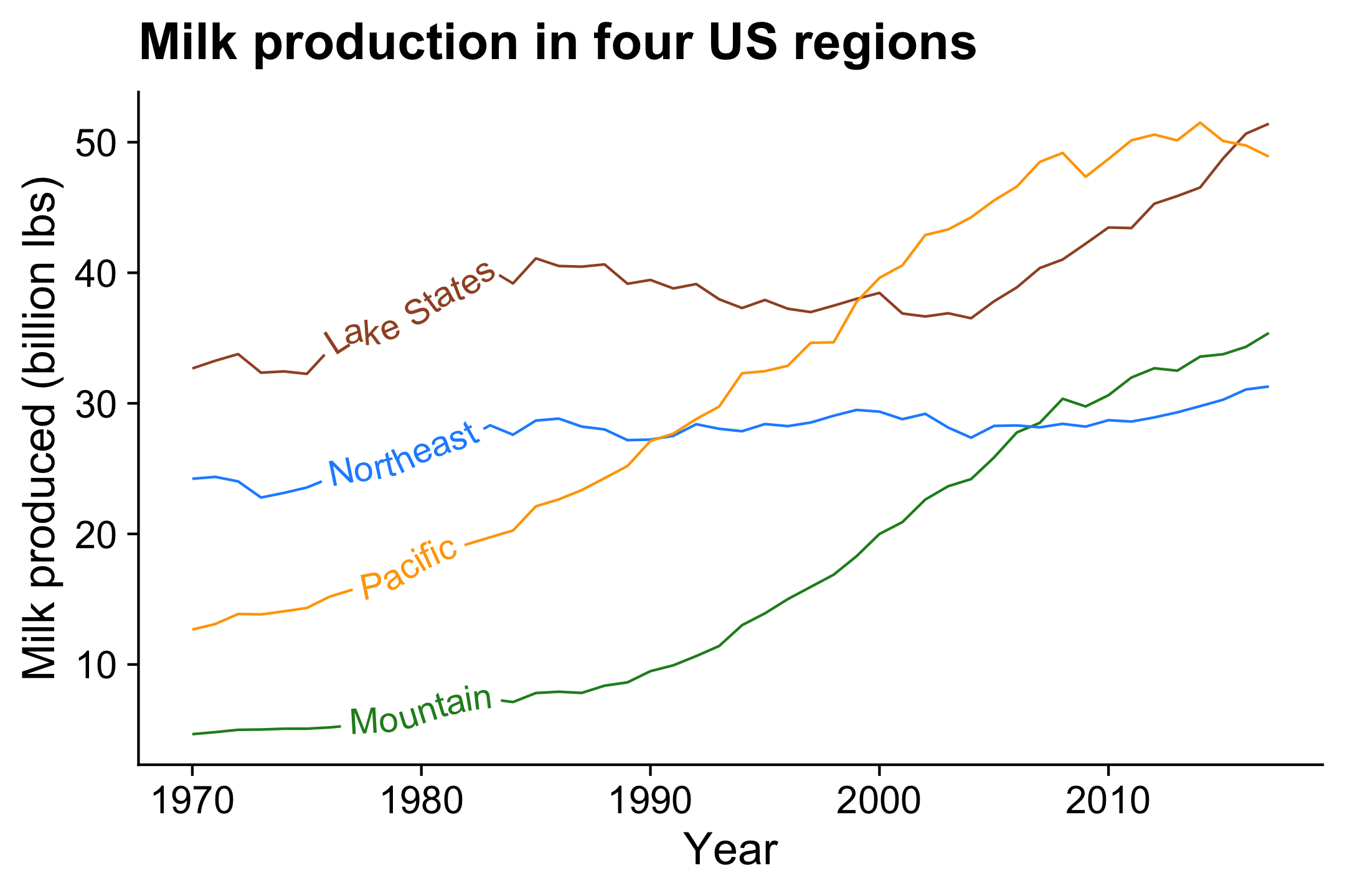
How to:
Directly label lines

library(geomtextpath)

# Format the data
milk_production %>%
  filter(
    region %in%
      c('Pacific', 'Northeast', 'Lake States', 'Mountain')
  ) %>%
  group_by(year, region) %>%
  summarise(milk_produced = sum(milk_produced)) %>%
  ungroup() %>%

  # Make the line plot
  ggplot() +
  geom_textline(
    aes(
      x = year,
      y = milk_produced,
      color = region,
      label = region,
      group = region
    ),
    size = 5,
    hjust = 0.15
  ) +
  scale_color_manual(
    values = c('sienna', 'forestgreen', 'dodgerblue', 'orange')
  ) +
  theme_half_open(font_size = 18) +
  # Remove legend
  theme(legend.position = 'none') +
  labs(
    x = 'Year',
    y = 'Milk produced (billion lbs)',
    title = 'Milk production in four US regions'
  )

Alternative:
Embed the labels!

Use {geomtextpath} package

(see this SO issue for other strategies)

How to: Stacked area

internet_region %>%
  mutate(numUsers = numUsers / 10^9) %>%
  ggplot() +
  geom_area(aes(x = year, y = numUsers, fill = region)) +
  # Nice colors from "viridis" library:
  scale_fill_viridis(discrete = TRUE) +
  # Sort the legend into 3 rows
  guides(
    fill = guide_legend(
      nrow = 3,
      byrow = FALSE
    )
  ) +
  theme_minimal_grid(font_size = 15) +
  theme(legend.position = 'bottom') +
  labs(
    x = 'Year',
    y = NULL,
    fill = 'Region',
    title = 'Number of internet users (billions)'
  )

Format the data

# Format the data
measles <- us_diseases %>%
  filter(
    disease == 'Measles',
    !state %in% c("Hawaii", "Alaska")
  ) %>%
  mutate(
    rate = (count / population) * 10000,
    state = fct_reorder(state, rate)
  ) %>%
  # Compute annual mean rate across all states
  group_by(year) %>%
  mutate(
    mean_rate = sum(count) / sum(population) * 10000
  )

Make all the state lines in light grey color

ggplot(measles) +
    geom_line(
        aes(x = year, y = rate, group = state),
        color = 'grey',
        alpha = 0.3
    ) +
    # Add reference line & label:
    geom_vline(xintercept = 1963, col = 'blue', linetype = 'dashed') +
    annotate(
        'text',
        x = 1964,
        y = 150,
        hjust = 0,
        label = 'Vaccine introduced in 1964',
        color = 'blue'
    ) +
    theme_minimal_grid(font_size = 18) +
    labs(y = 'Cases per 10,000 people')

How to:
Average line overlay

Now overlay the annual mean line

ggplot(measles) +
  geom_line(
    aes(x = year, y = rate, group = state),
    color = 'grey',
    alpha = 0.3
  ) +
  geom_line(
    aes(x = year, y = mean_rate),
    size = 0.8
  ) +
  # Add US mean label
  annotate(
    'text',
    x = 1945,
    y = 55,
    hjust = 0,
    label = 'US Mean'
  ) +
  # Add reference line & label
  geom_vline(xintercept = 1963, col = 'blue', linetype = 'dashed') +
  annotate(
    'text',
    x = 1964,
    y = 150,
    hjust = 0,
    label = 'Vaccine introduced in 1964',
    color = 'blue'
  ) +
  theme_minimal_grid(font_size = 18) +
  labs(y = 'Cases per 10,000 people')

How to:
Average line overlay

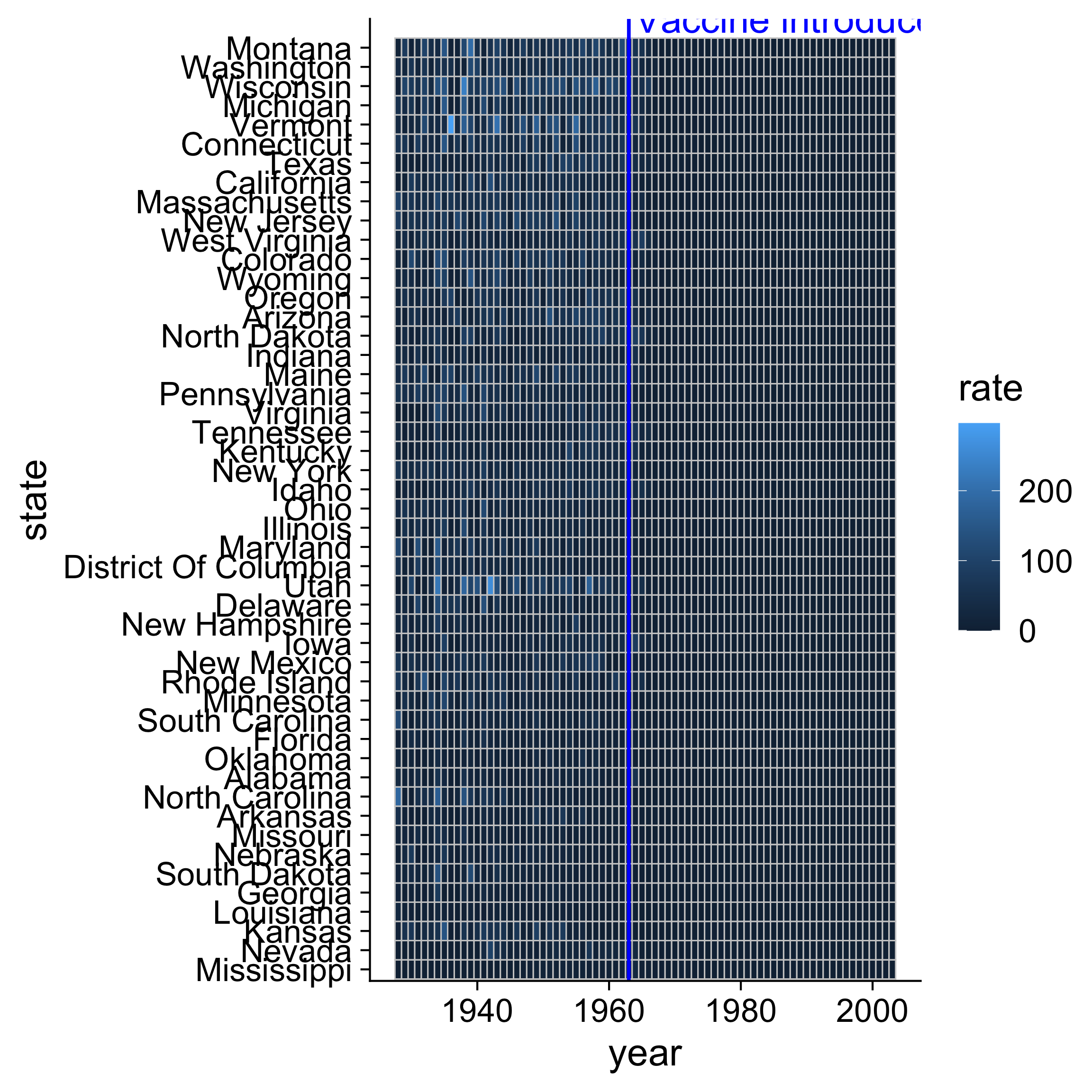
Create main grid with geom_tile()

ggplot(measles) +
  geom_tile(
    aes(x = year, y = state, fill = rate),
    color = 'grey80'
  ) +
  # Add reference line & label
  geom_vline(
    xintercept = 1963,
    col = 'blue'
  ) +
  annotate(
    'text',
    x = 1964,
    y = 50.5,
    hjust = 0,
    label = 'Vaccine introduced in 1964',
    color = 'blue'
  )

How to: Heat map

Adjust scales and adjust theme

ggplot(measles) +
  geom_tile(aes(x = year, y = state, fill = rate), color = 'grey80') +
  # Add reference line & label
  geom_vline(xintercept = 1963, col = 'blue') +
  annotate(
    'text',
    x = 1964,
    y = 50.5,
    hjust = 0,
    label = 'Vaccine introduced in 1964',
    color = 'blue'
  ) +
  # Adjust scales
  scale_x_continuous(expand = c(0, 0)) +
  scale_fill_viridis(
    option = 'inferno',
    direction = -1
  ) +
  # Adjust theme
  theme_minimal() +
  theme(
    panel.grid = element_blank(),
    legend.position = 'bottom',
    text = element_text(size = 10)
  ) +
  coord_cartesian(clip = 'off') +
  labs(
    x = NULL,
    y = NULL,
    fill = 'Cases per 10,000 people',
    title = 'Measles'
  )

Color scale is linear in this chart

Adjust scales and adjust theme

ggplot(measles) +
  geom_tile(aes(x = year, y = state, fill = rate), color = 'grey80') +
  # Add reference line & label
  geom_vline(xintercept = 1963, col = 'blue') +
  annotate(
    'text',
    x = 1964,
    y = 50.5,
    hjust = 0,
    label = 'Vaccine introduced in 1964',
    color = 'blue'
  ) +
  # Adjust scales
  scale_x_continuous(expand = c(0, 0)) +
  scale_fill_viridis(
    option = 'inferno',
    direction = -1,
    trans = 'sqrt'
  ) +
  # Modify legend color bar
  guides(
    fill = guide_colorbar(
      title.position = 'top',
      reverse = TRUE
    )
  ) +
  # Adjust theme
  theme_minimal() +
  theme(
    panel.grid = element_blank(),
    legend.position = 'bottom',
    text = element_text(size = 10)
  ) +
  coord_cartesian(clip = 'off') +
  labs(
    x = NULL,
    y = NULL,
    fill = 'Cases per 10,000 people',
    title = 'Measles'
  )

Non-linear color scale
helps with large variations

Your turn

Use the us_covid data frame to explore ways to visualize the number of daily cases using:

1. A labeled line chart
2. A stacked area chart
3. A heat map

us_covid <- read_csv(file.path(
  'data',
  'us_covid.csv'
))

head(us_covid)

#> # A tibble: 6 × 7
#>   date         day state   cases_daily deaths_daily cases_total deaths_total
#>   <date>     <dbl> <chr>         <dbl>        <dbl>       <dbl>        <dbl>
#> 1 2020-01-23     1 Alabama           0            0           0            0
#> 2 2020-01-24     2 Alabama           0            0           0            0
#> 3 2020-01-25     3 Alabama           0            0           0            0
#> 4 2020-01-26     4 Alabama           0            0           0            0
#> 5 2020-01-27     5 Alabama           0            0           0            0
#> 6 2020-01-28     6 Alabama           0            0           0            0

Two other examples for showing
change across multiple categories

Seasonal chart

Source: http://r-statistics.co/Top50-Ggplot2-Visualizations-MasterList-R-Code.html#Seasonal%20Plot

Sankey chart

Source: https://flowcharts.llnl.gov/

Would you consider purchasing an electric car?

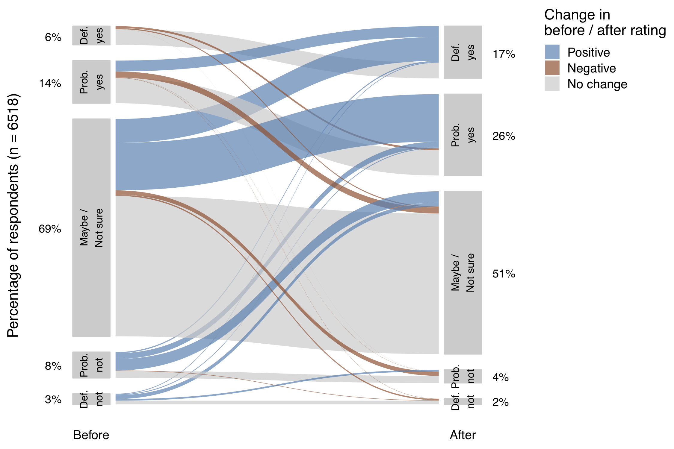
Roberson, Laura A. & Helveston, J.P. (2020) “Electric vehicle adoption: can short experiences lead to big change?,” Environmental Research Letters. 15(0940c3).
Made using the ggforce package