Visualizing Information

EMSE 4572/6572: Exploratory Data Analysis

John Paul Helveston

October 07, 2026

References:

- Data Viz “Cheat Sheet”

- Data Viz Reference Page

From here

“Having word processing software
doesn’t make us great writers.”

— Stephen Few

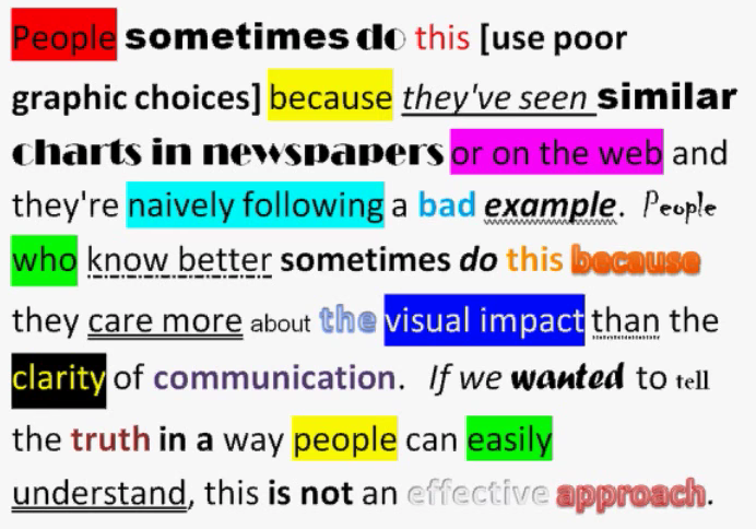
We don’t write paragraphs like this

Image from Few (2012, pg. 227)

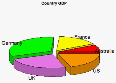
So don’t make
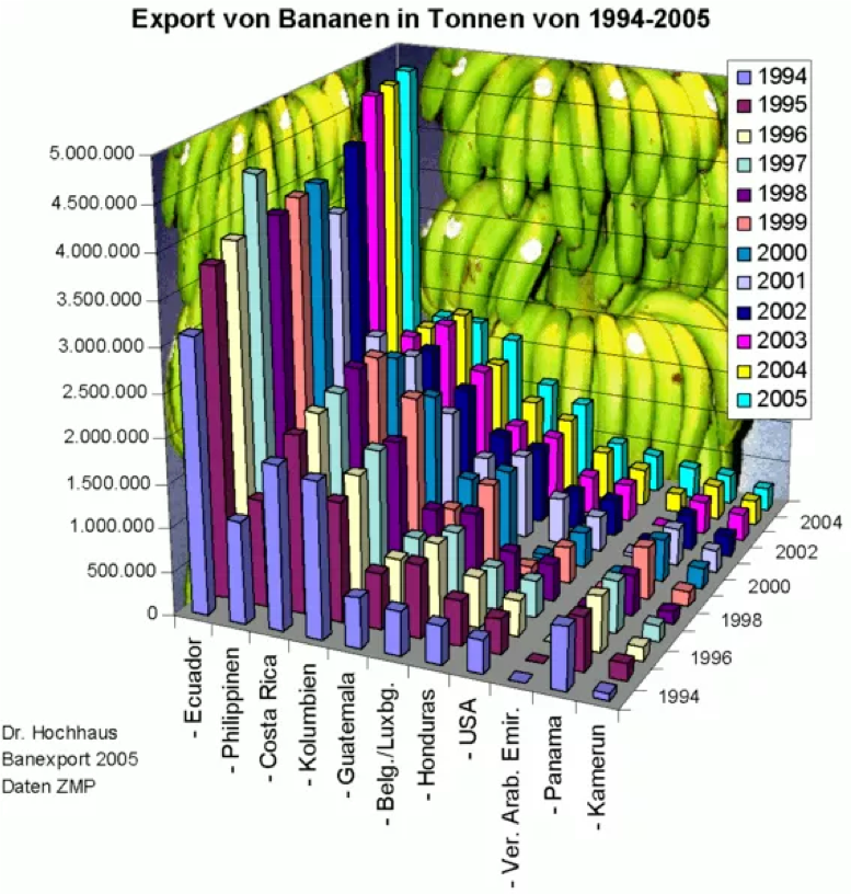
graphs like this

Image from excelcharts.com

Week 7: Visualizing Information

1. The Human Visual-Memory System

2. The Psychology of Data Viz

3. 10 Data Viz Best Practices

4. Making a (good) ggplot

Week 7: Visualizing Information

1. The Human Visual-Memory System

2. The Psychology of Data Viz

3. 10 Data Viz Best Practices

4. Making a (good) ggplot

Good visualizations optimize for
the human visual-memory system

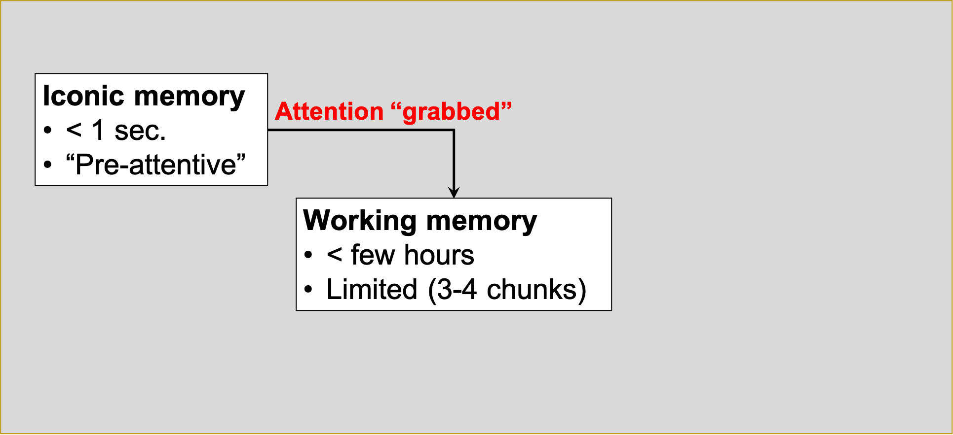
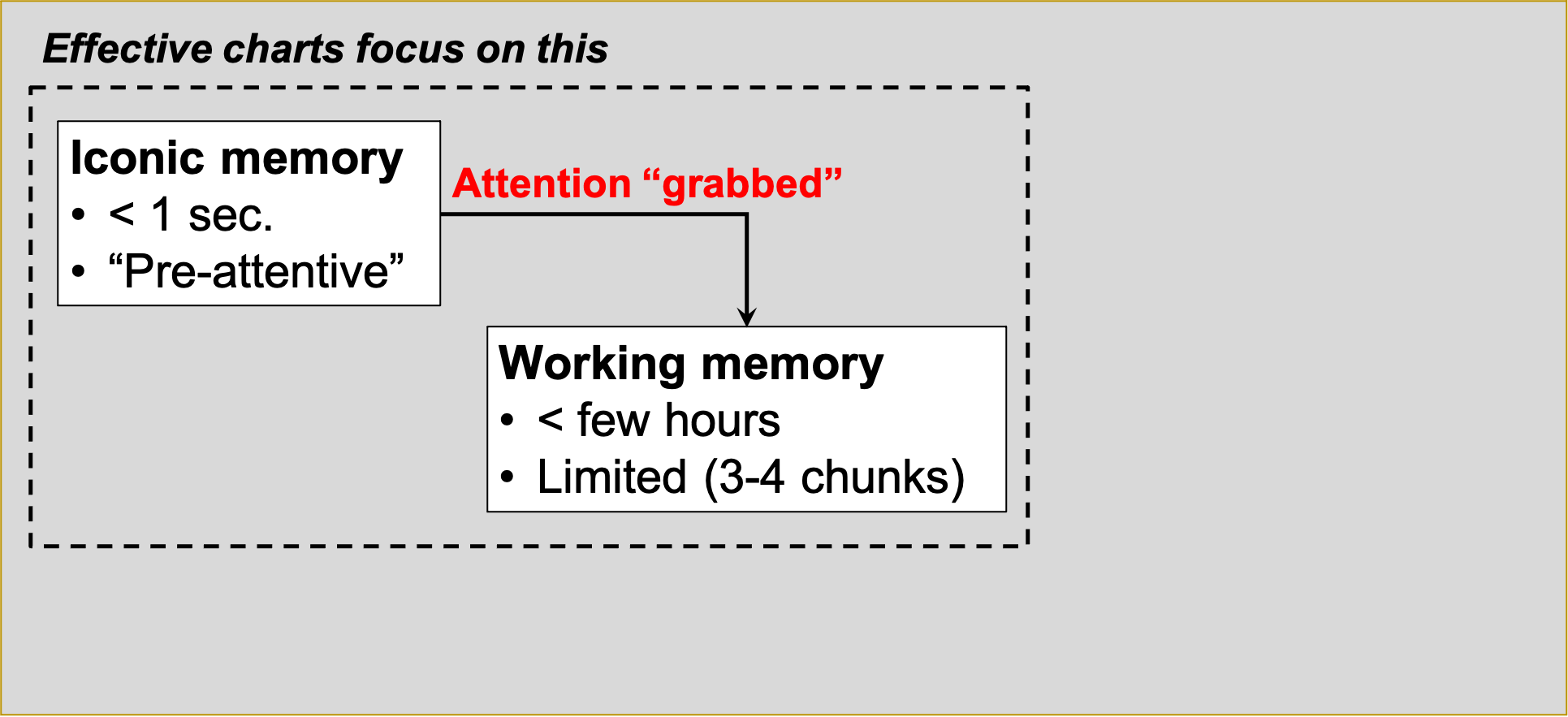
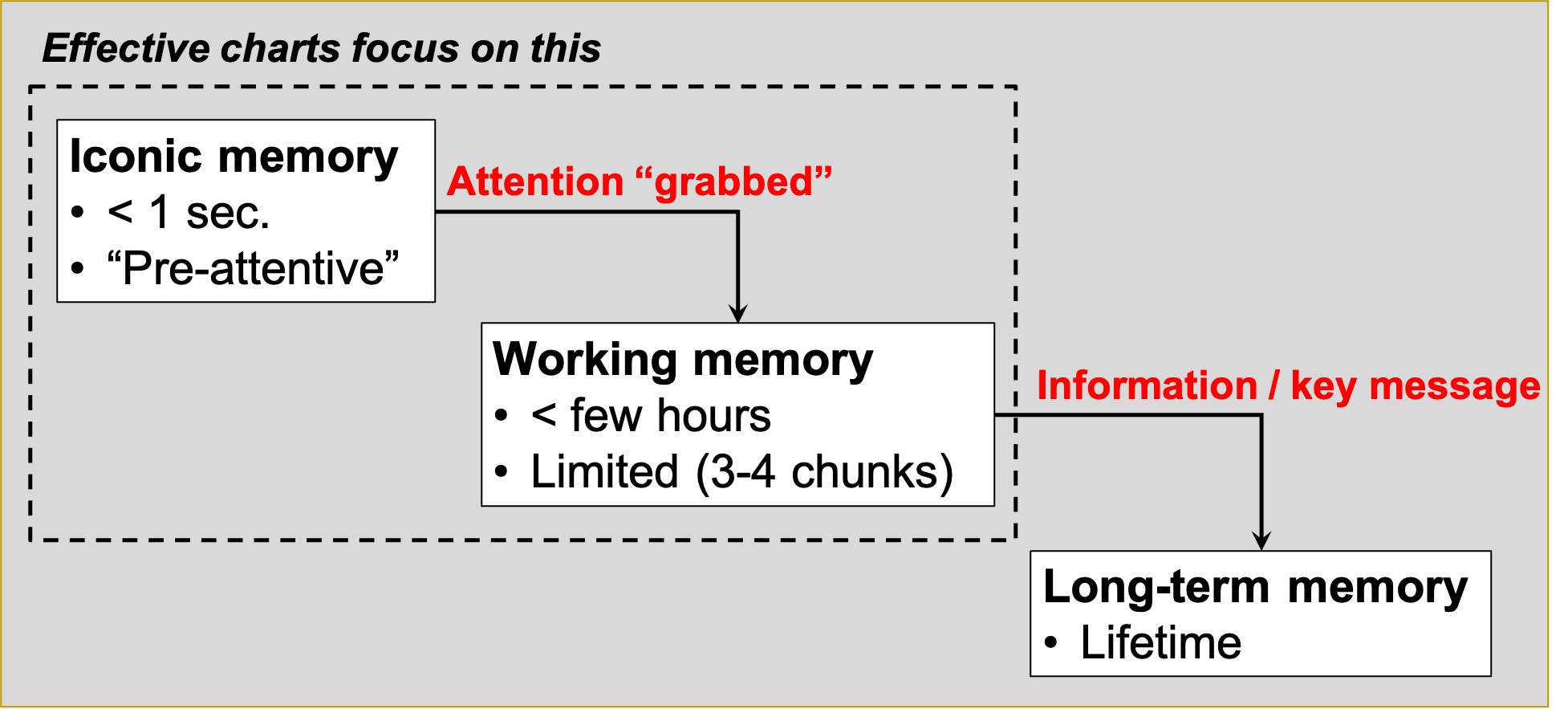
A (very) simplified model of the visual-memory system

A (very) simplified model of the visual-memory system

A (very) simplified model of the visual-memory system

A (very) simplified model of the visual-memory system

Two objectives of effective charts:

1. Grab & direct attention (iconic memory)

2. Reduce processing demands (working memory)

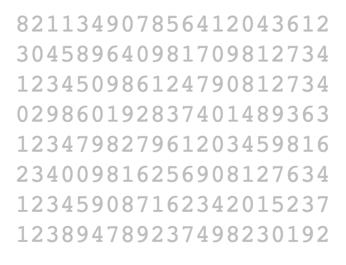
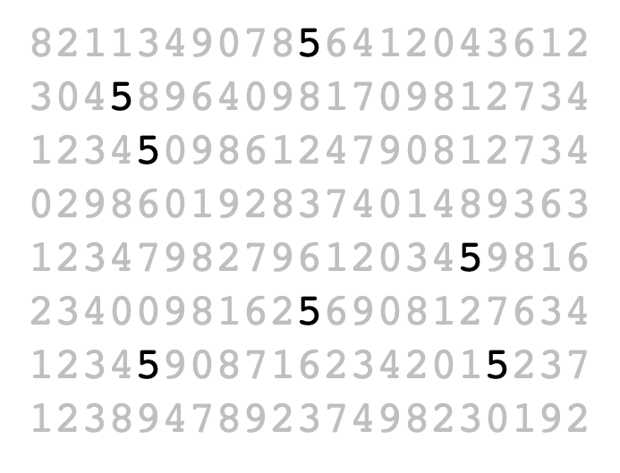
The power of pre-attentive processing

Count all the “5”’s

The power of pre-attentive processing

Count all the “5”’s

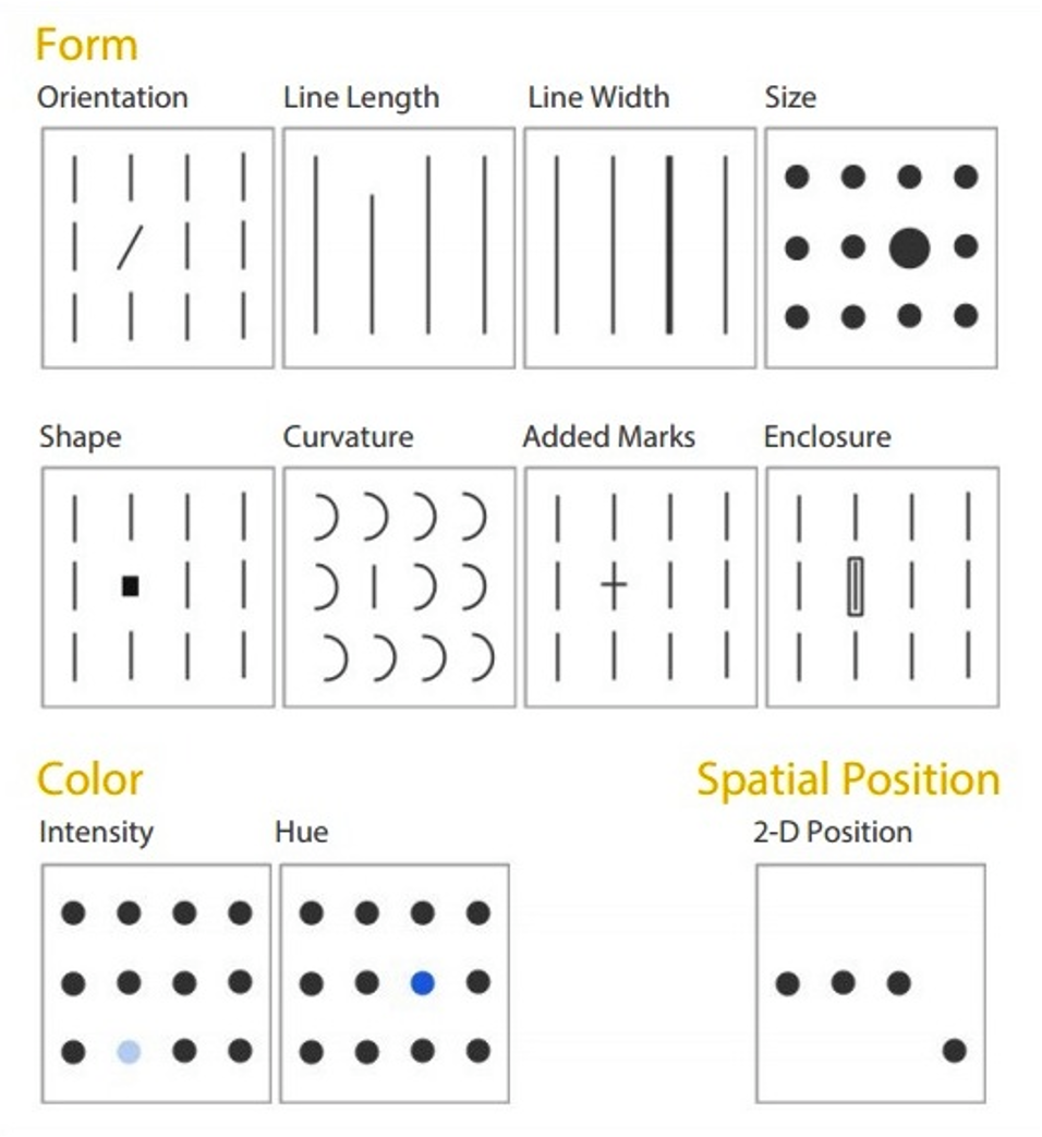
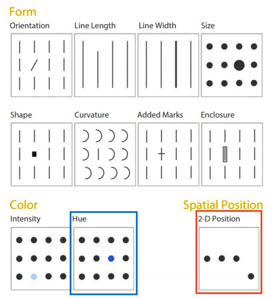
Pre-attentive attributes

Pre-attentive attributes

Numerical (ratio) data

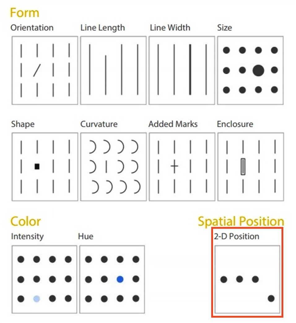
Pre-attentive attributes

Numerical (ratio) data
Categorical (ordinal) data

Not all pre-attentive attributes are equal

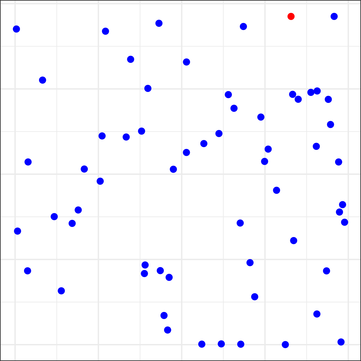
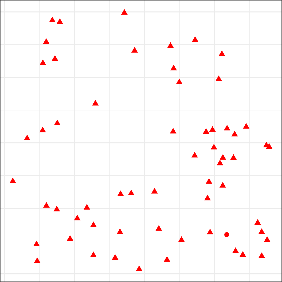
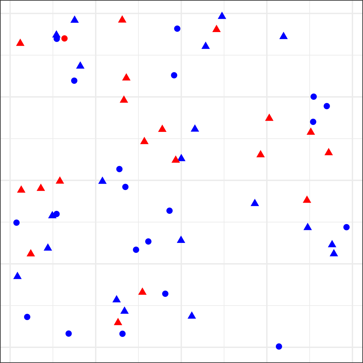
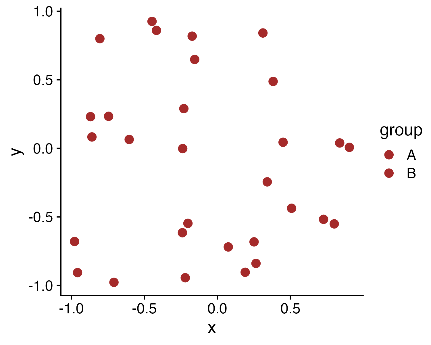
Where is the red dot?

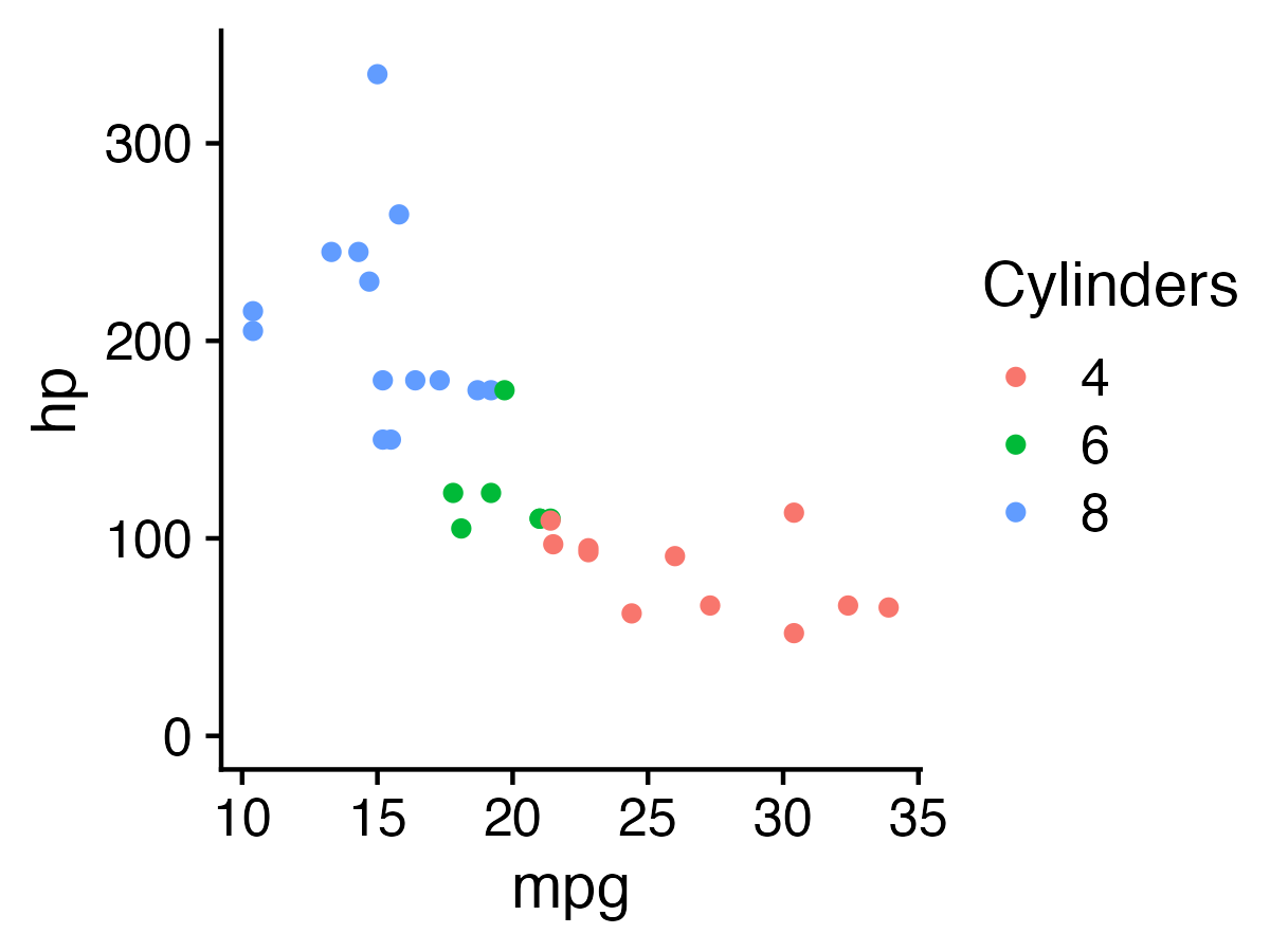
For categorical data:

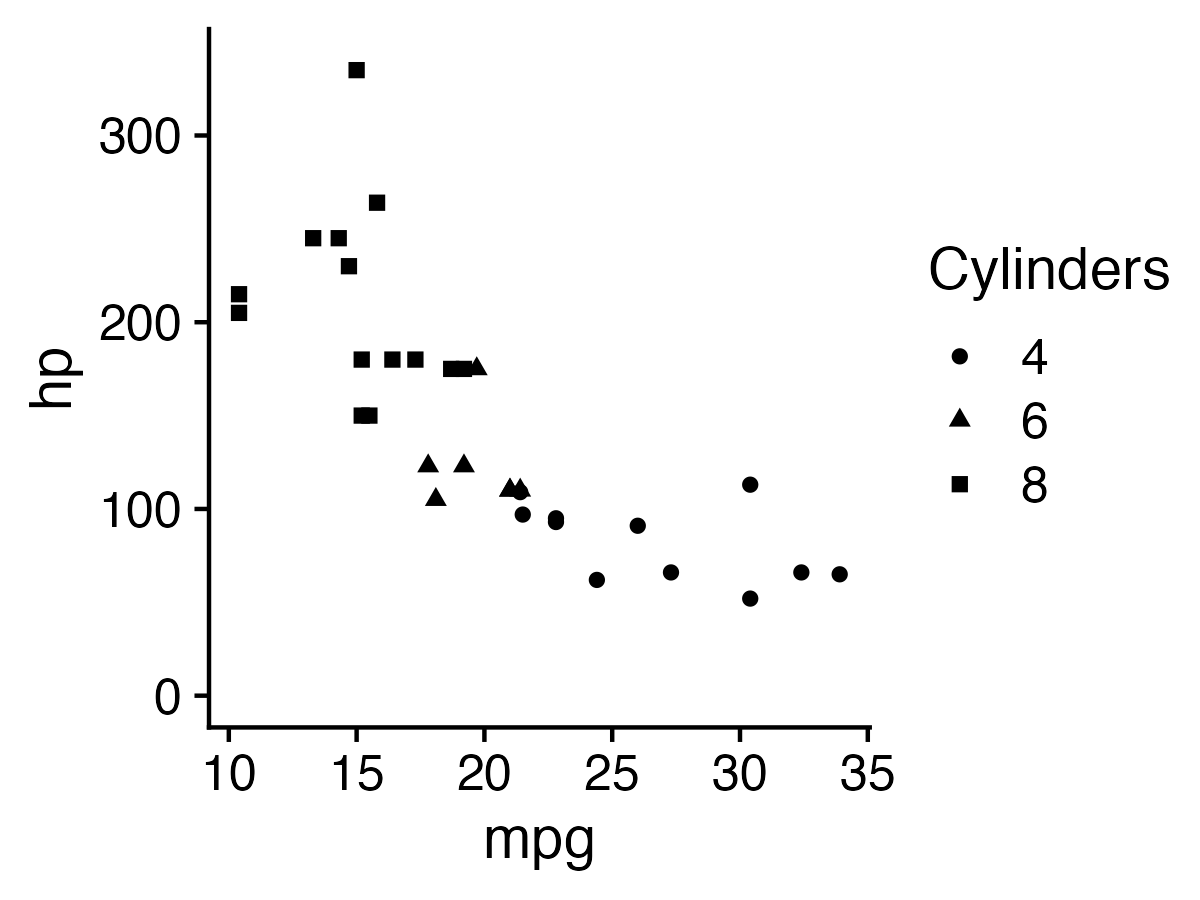
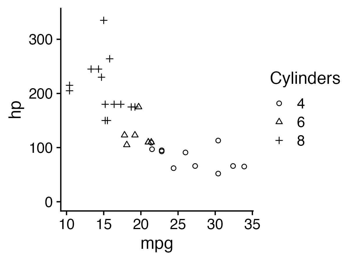
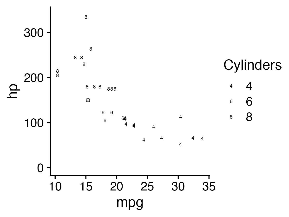
1. Hue (color) > shape

2. Less is more (stay in working memory!)

Week 7: Visualizing Information

1. The Human Visual-Memory System

2. The Psychology of Data Viz

3. 10 Data Viz Best Practices

4. Making a (good) ggplot

Much of the content in this section is from
John Rauser’s talk on YouTube

(Always cite your sources)

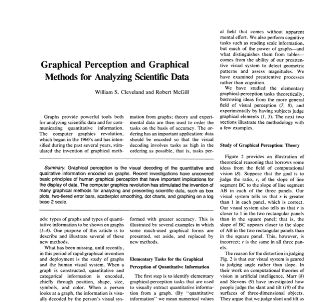
Cleveland, W. S., & McGill, R. (1985). Graphical perception and graphical methods for analyzing scientific data. Science, New Series, 229(4716), 828-833.

Cleveland’s operations of pattern perception:

1. Estimation

2. Assembly

3. Detection

Cleveland’s operations of pattern perception:

1. Estimation ——–>

2. Assembly

3. Detection

• Discrimination (X equal to Y?)

• Ranking (X greater than Y?)

• Ratioing (X double Y?)

Estimation: Hierarchy for numerical data

More Accurate

Less Accurate

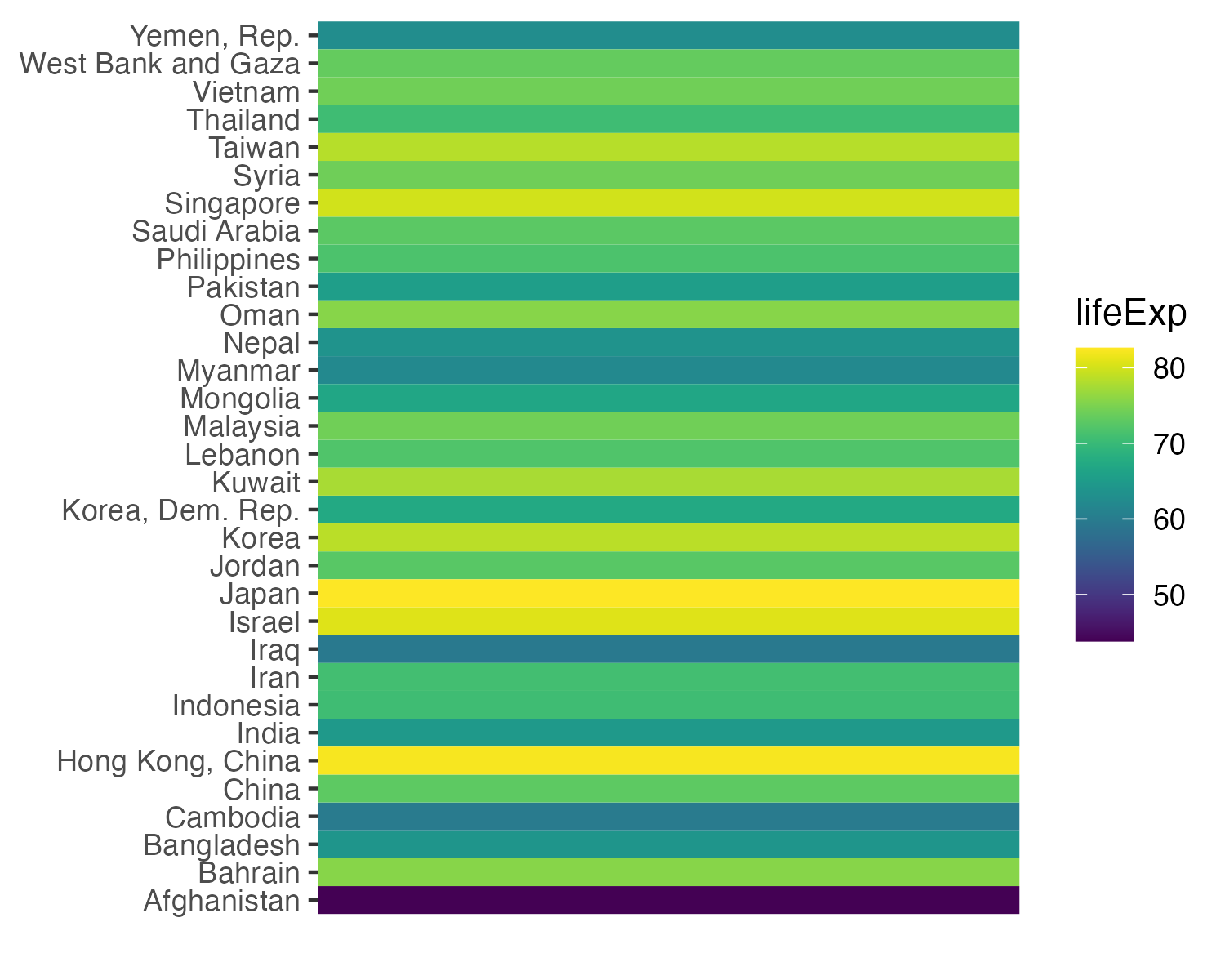
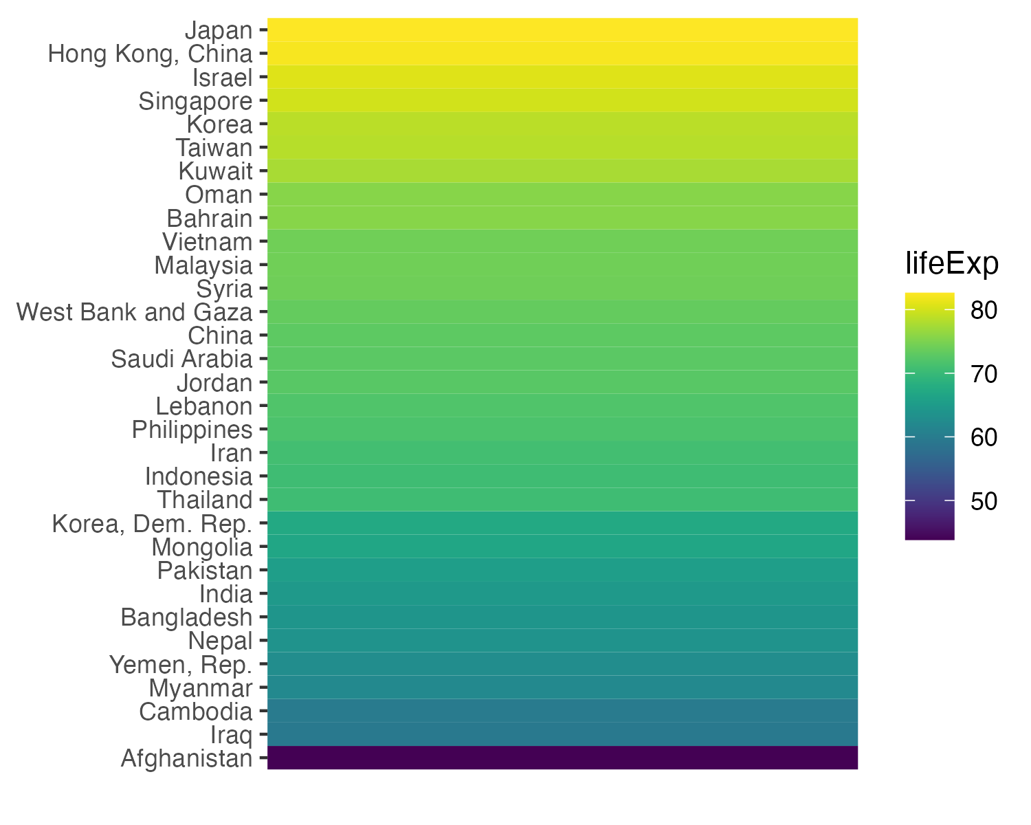
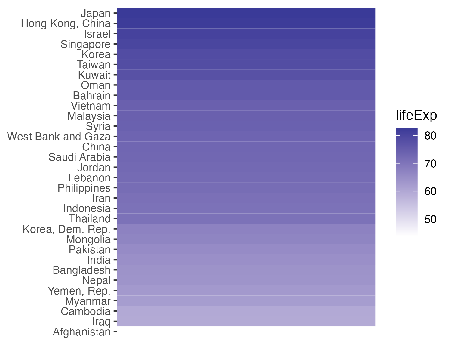
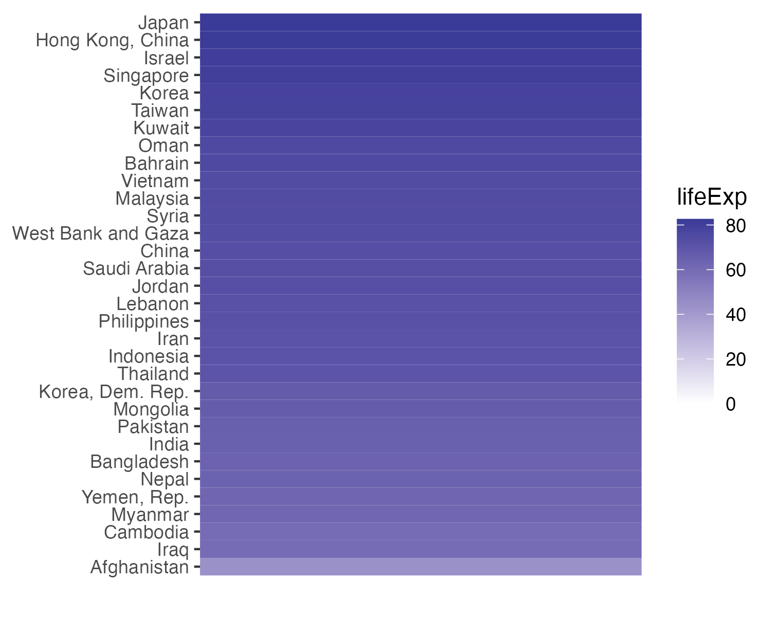
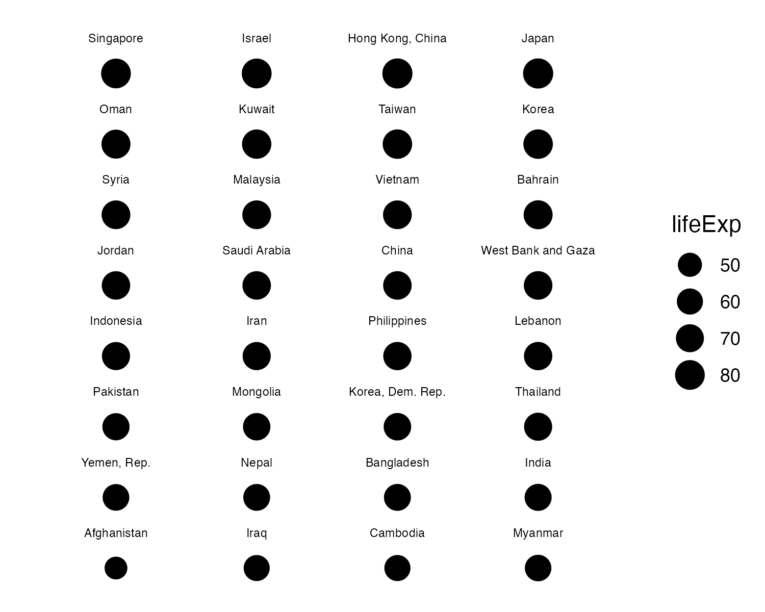
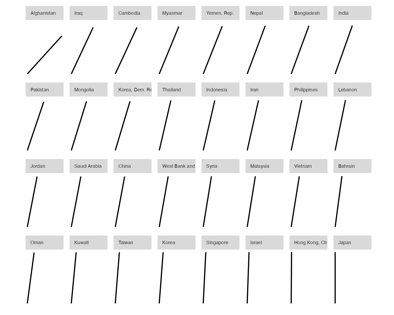
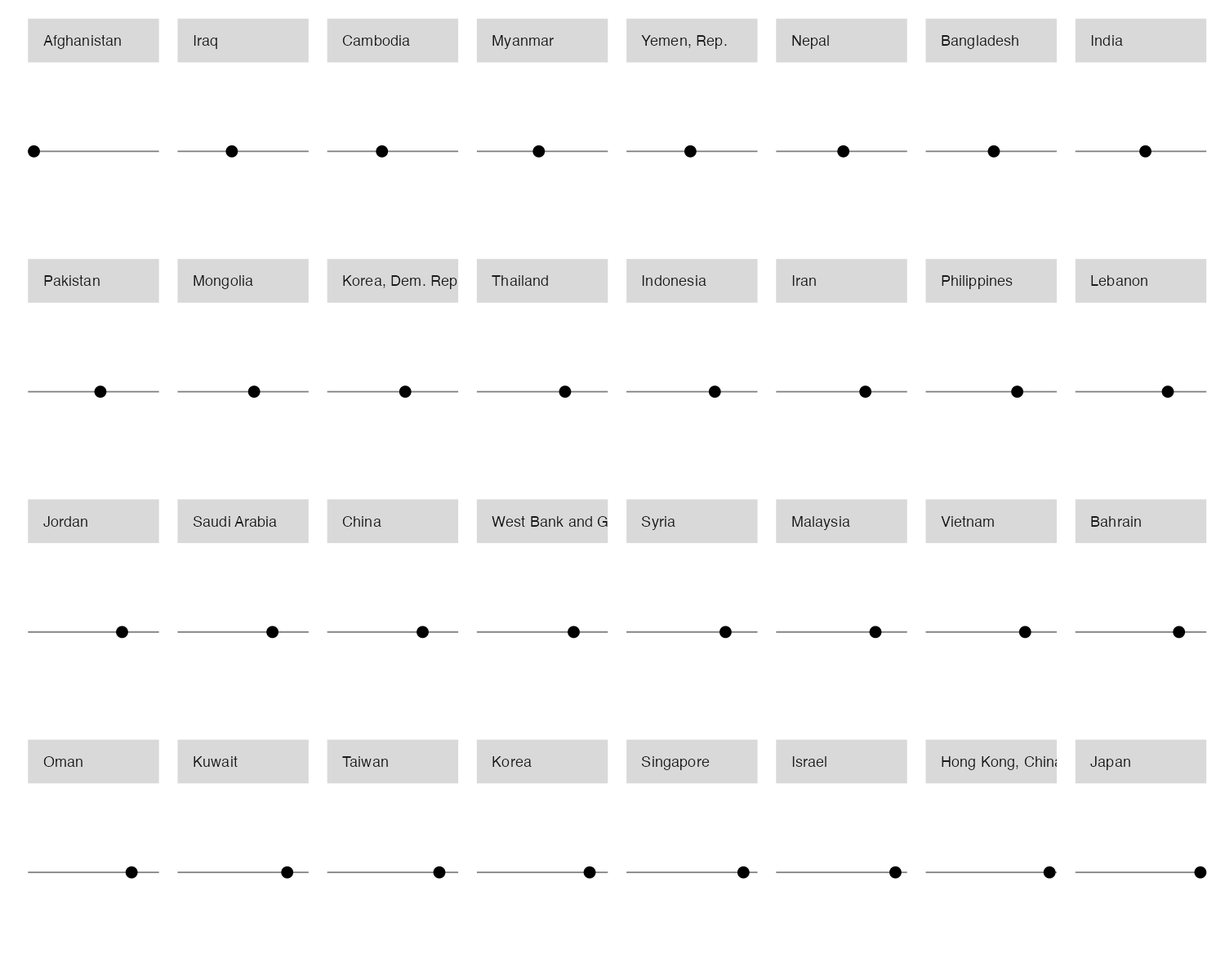
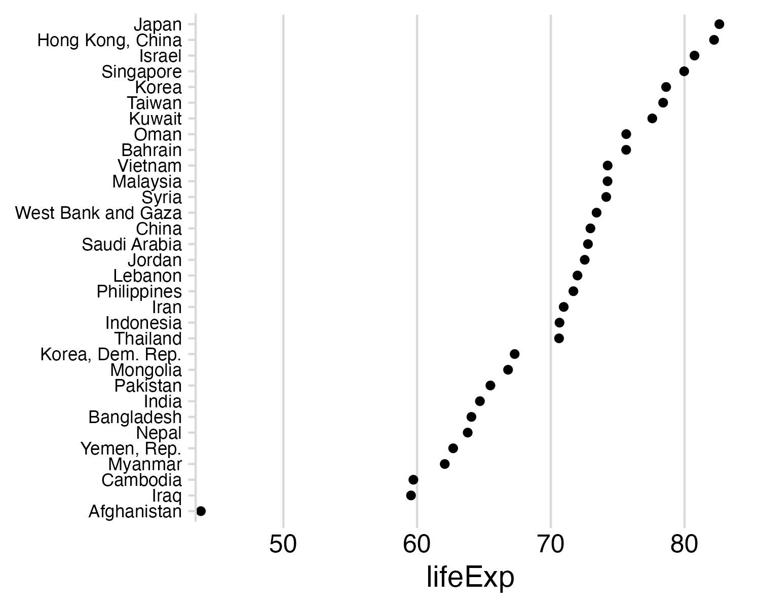
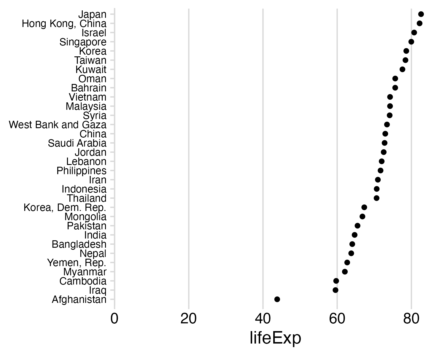
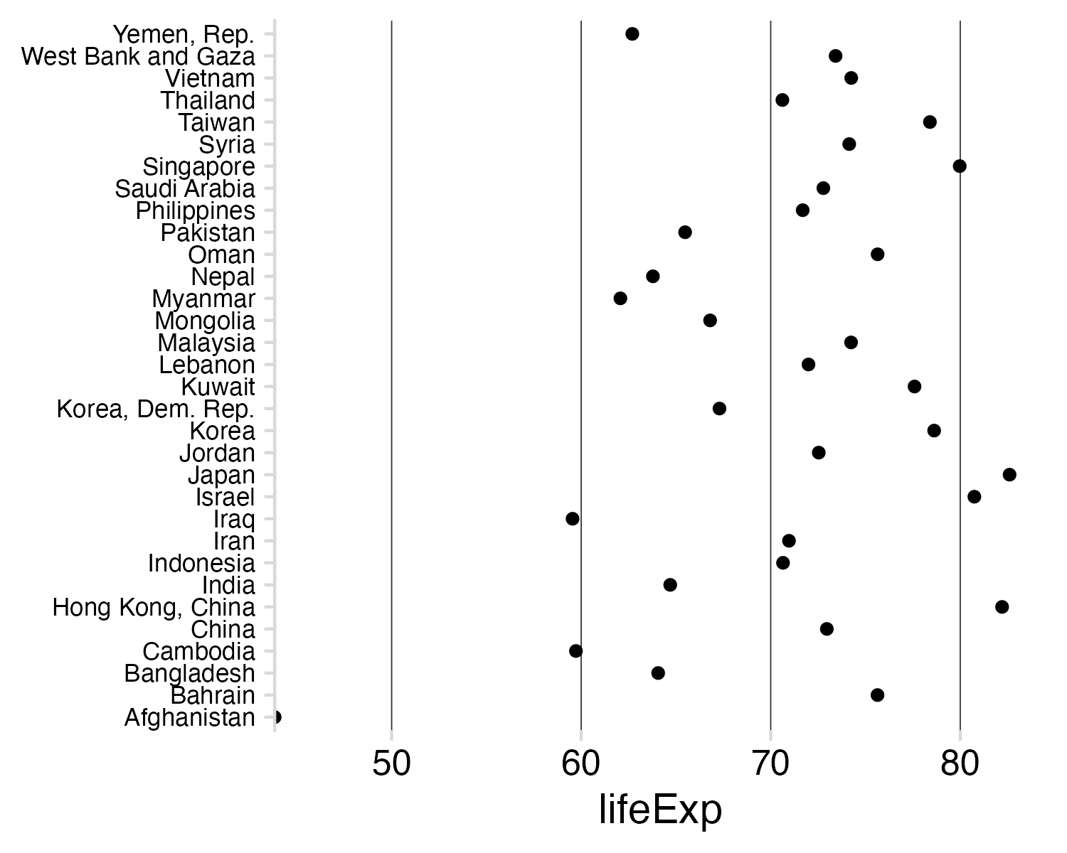
Example: Life expectancy in countries in Asia

#>               country lifeExp
#> 1         Afghanistan  43.828
#> 2                Iraq  59.545
#> 3            Cambodia  59.723
#> 4             Myanmar  62.069
#> 5         Yemen, Rep.  62.698
#> 6               Nepal  63.785
#> 7          Bangladesh  64.062
#> 8               India  64.698
#> 9            Pakistan  65.483
#> 10           Mongolia  66.803
#> 11   Korea, Dem. Rep.  67.297
#> 12           Thailand  70.616
#> 13          Indonesia  70.650
#> 14               Iran  70.964
#> 15        Philippines  71.688
#> 16            Lebanon  71.993
#> 17             Jordan  72.535
#> 18       Saudi Arabia  72.777
#> 19              China  72.961
#> 20 West Bank and Gaza  73.422

1. Position on a common scale
2. Position on
   non-aligned scales
3. Length
4. Angle
5. Area
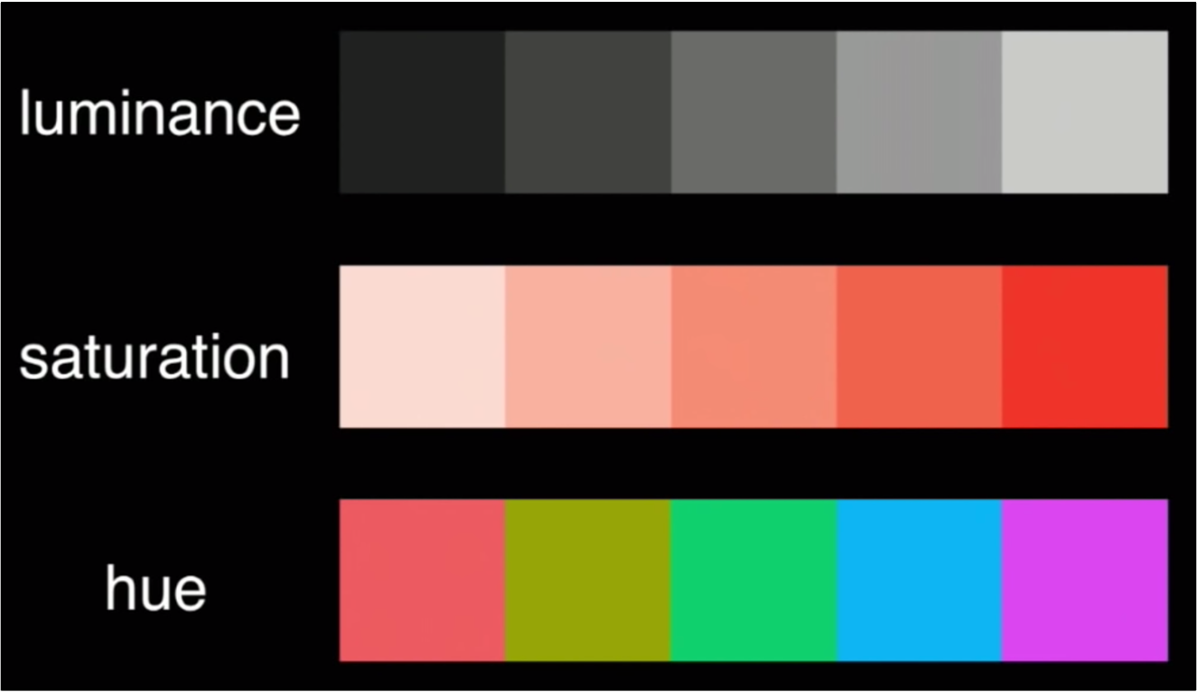
6. Color saturation
7. Color hue

1. Position on a common scale
2. Position on
   non-aligned scales
3. Length
4. Angle
5. Area
6. Color saturation
7. Color hue

• / Discriminate
• / Rank
• Ratio

1. Position on a common scale
2. Position on
   non-aligned scales
3. Length
4. Angle
5. Area
6. Color saturation
7. Color hue

Sorting helps a bit…

• / Discriminate
• / Rank
• Ratio

1. Position on a common scale
2. Position on
   non-aligned scales
3. Length
4. Angle
5. Area
6. Color saturation
7. Color hue

• / Discriminate
• / Rank
• Ratio

1. Position on a common scale
2. Position on
   non-aligned scales
3. Length
4. Angle
5. Area
6. Color saturation
7. Color hue

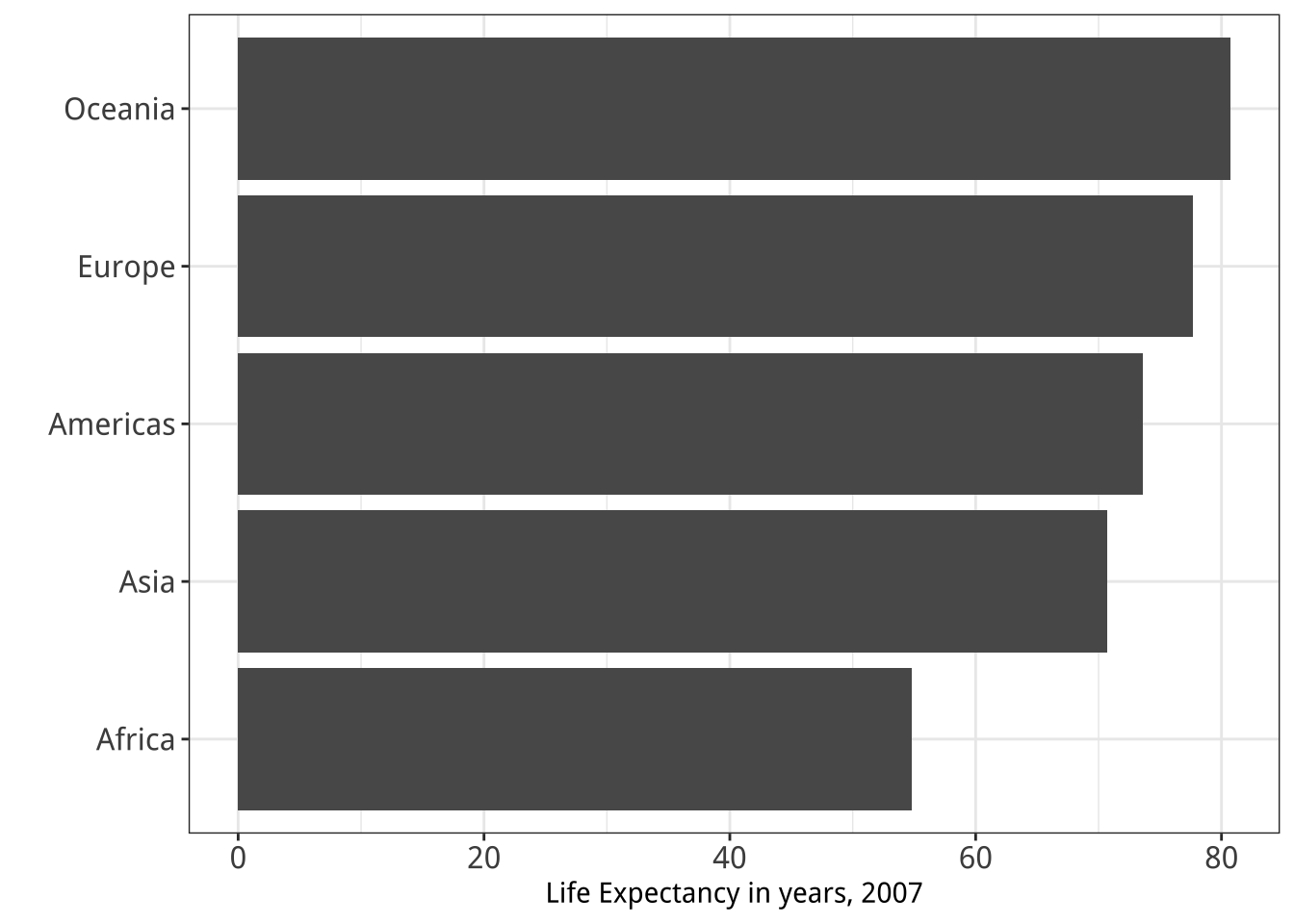
Align to 0 scale:

• / Discriminate
• / Rank
• / Ratio

1. Position on a common scale
2. Position on
   non-aligned scales
3. Length
4. Angle
5. Area
6. Color saturation
7. Color hue

• / Discriminate
• / Rank
• / Ratio

1. Position on a common scale
2. Position on
   non-aligned scales
3. Length
4. Angle
5. Area
6. Color saturation
7. Color hue

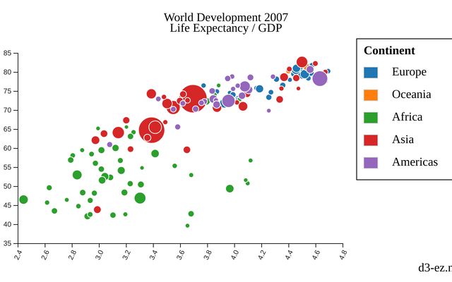
Area works okay for “bubble” charts

1. Position on a common scale
2. Position on
   non-aligned scales
3. Length
4. Angle
5. Area
6. Color saturation
7. Color hue

• / Discriminate
• Rank
• / Ratio

1. Position on a common scale
2. Position on
   non-aligned scales
3. Length
4. Angle
5. Area
6. Color saturation
7. Color hue

1. Position on a common scale
2. Position on
   non-aligned scales
3. Length
4. Angle
5. Area
6. Color saturation
7. Color hue

• / Discriminate
• / Rank
• Ratio

1. Position on a common scale
2. Position on
   non-aligned scales
3. Length
4. Angle
5. Area
6. Color saturation
7. Color hue

• / Discriminate
• / Rank
• Ratio

1. Position on a common scale
2. Position on
   non-aligned scales
3. Length
4. Angle
5. Area
6. Color saturation
7. Color hue

• Discriminate
• Rank
• Ratio

1. Position on a common scale
2. Position on
   non-aligned scales
3. Length
4. Angle
5. Area
6. Color saturation
7. Color hue

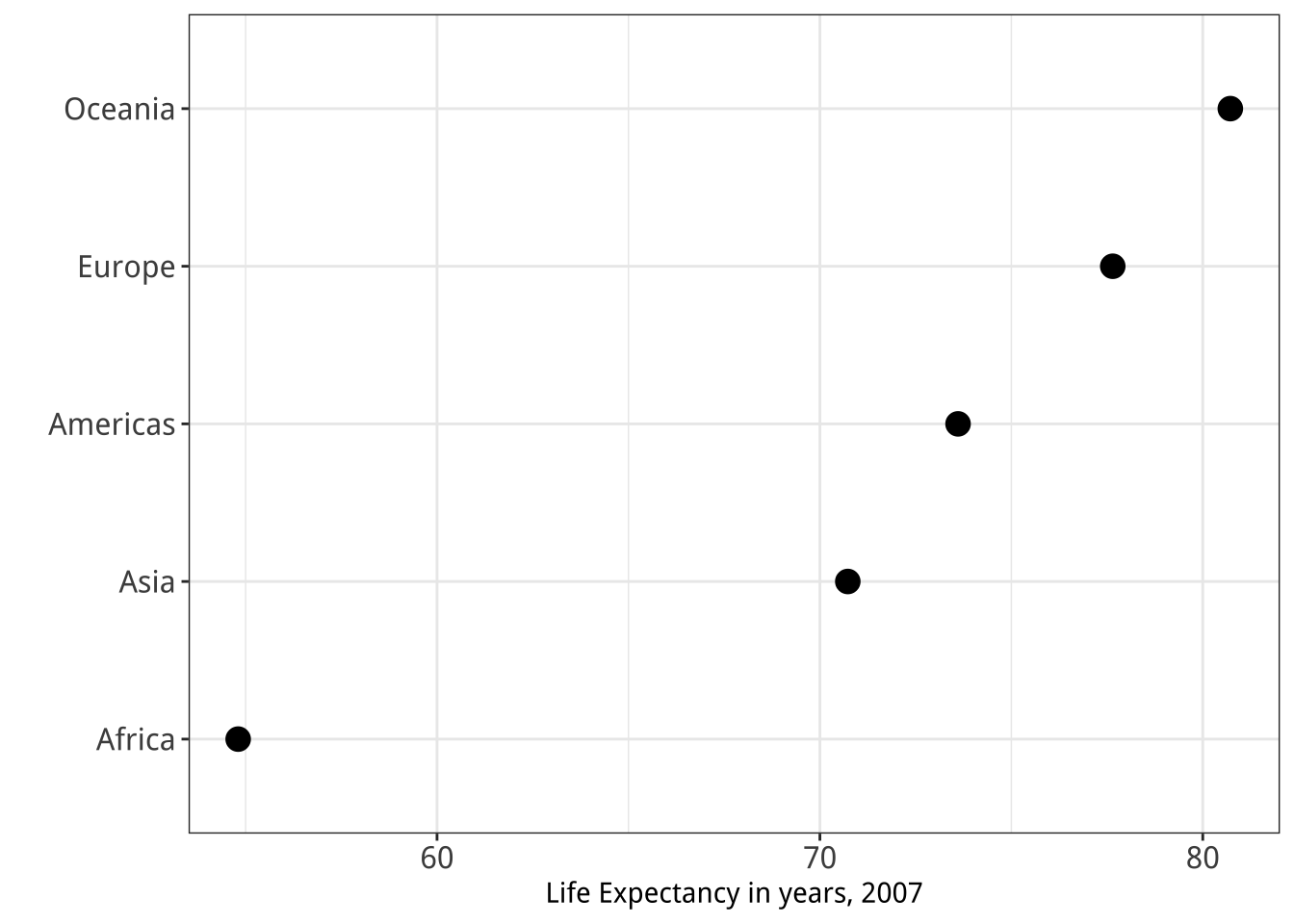
No need to scale to 0:

• Lowers resolution
• Isn’t needed for accurate ratioing

1. Position on a common scale
2. Position on
   non-aligned scales
3. Length
4. Angle
5. Area
6. Color saturation
7. Color hue

Sorting still matters!

Cleveland’s operations of pattern perception:

1. Estimation

2. Assembly

3. Detection

Cleveland’s operations of pattern perception:

1. Estimation

2. Assembly ——–>

3. Detection

The grouping of graphical elements

Assembly: Gestalt Psychology

The whole has a reality that is entirely separate from the parts

Reification

Emergence

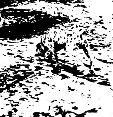
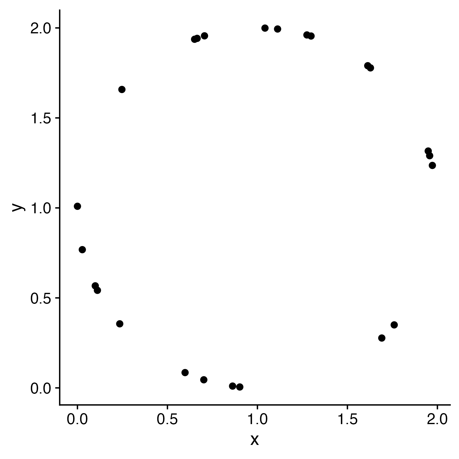
Law of Closure

Our minds fill in the missing information

Prägnanz

We strongly prefer to interpret stimuli as regular, simple, and orderly

Prägnanz

This should cause you cognitive pain

It’s the graphical equivalent of this:

Prägnanz

This makes our brains happy

Law of Continuity

We will group together objects that follow an established direction

Law of Continuity

We will group together objects that follow an established direction

Law of Similarity

We see elements that are physically similar as part of the same object

Law of Similarity

We see elements that are physically similar as part of the same object

Law of Similarity

We see elements that are physically similar as part of the same object

Law of Similarity

We see elements that are physically similar as part of the same object

Law of Proximity

We tend to see elements that are physically near each other as part of the same object

Law of Proximity

We tend to see elements that are physically near each other as part of the same object

Law of Proximity

We tend to see elements that are physically near each other as part of the same object

Cleveland’s operations of pattern perception:

1. Estimation

2. Assembly

3. Detection

Estimation: Hierarchy for numerical data

More Accurate

Less Accurate

Assembly: Gestalt Psychology

Law of Closure	Prägnanz	Law of Continuity	Law of Similarity	Law of Proximity
Fill in the missing information	We like regular, simple, and orderly	Group together objects with established direction	Physically similar = same object	Physically near = same object

Cleveland’s operations of pattern perception:

1. Estimation

2. Assembly

3. Detection ——–>

Recognizing that a geometric
object encodes a physical value

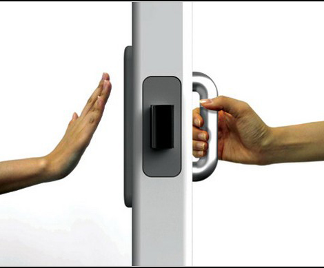
Norman door (n.):

1. A door where the design tells you to do the opposite of what you’re actually supposed to do.

2. A door that gives the wrong signal and needs a sign to correct it.

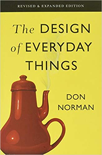
Norman door

Non-Norman door

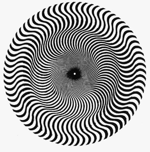
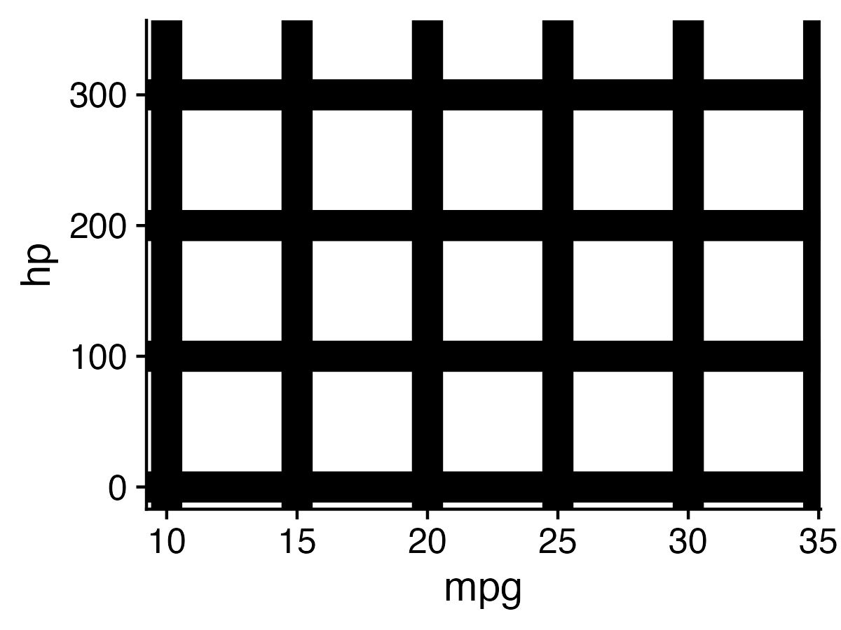
The white circles you see at the intersections is called the “Hermann Grid illusion”

05:00

Break!

Stand up, Move around, Stretch!

Week 7: Visualizing Information

1. The Human Visual-Memory System

2. The Psychology of Data Viz

3. 10 Data Viz Best Practices

4. Making a (good) ggplot

10 Data Viz Best Practices

1. Remove chart chunk
2. Don’t make 3D plots*
3. Don’t lie
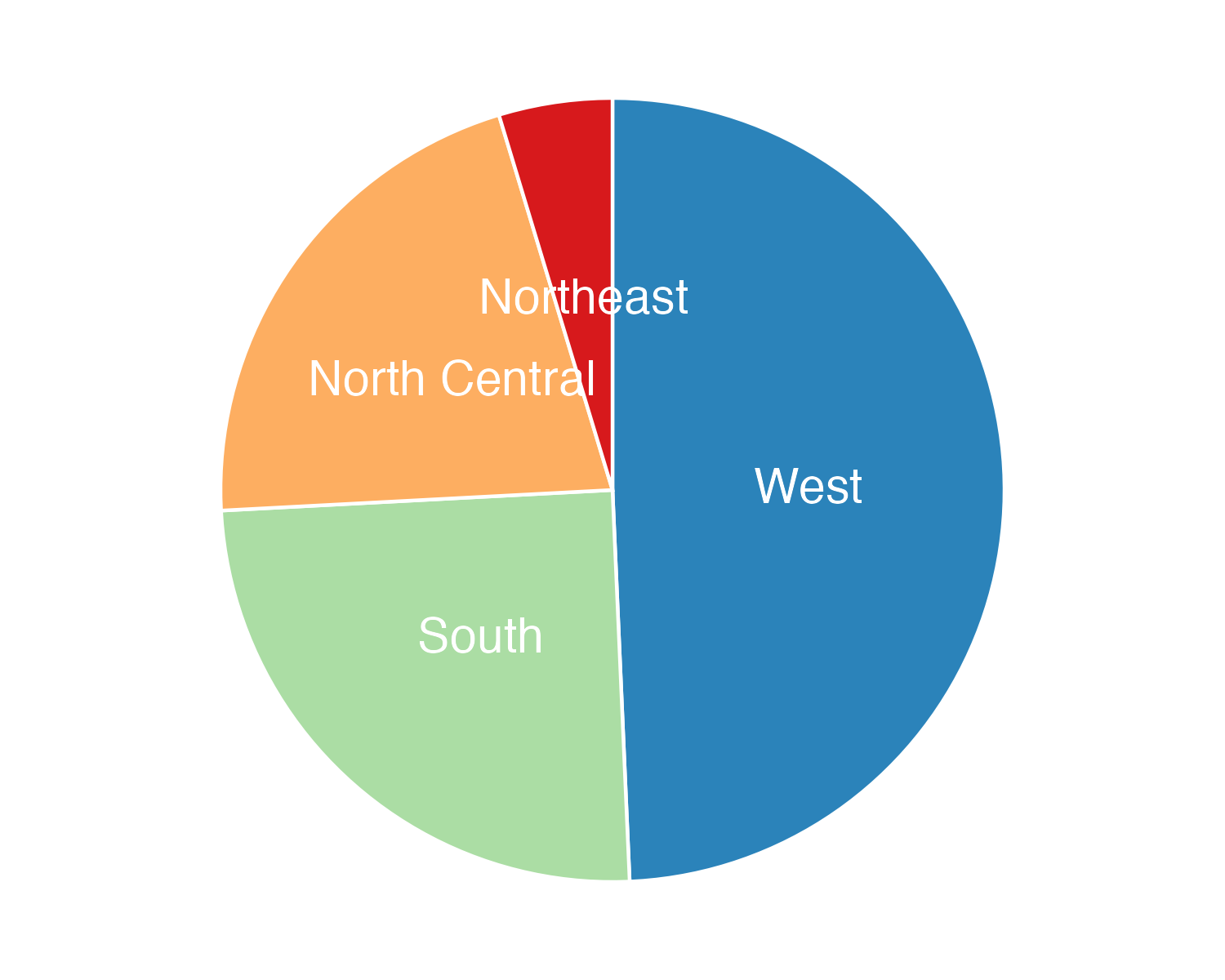
4. Don’t use pie charts for proportions*
5. Don’t stack bars*
6. Rotate and sort categorical axes*
7. Eliminate legends & directly label geoms*
8. Don’t use pattern fills
9. Don’t use red & green together
10. Consider tables for small data sets

*most of the time

10 Data Viz Best Practices

1. Remove chart chunk
2. Don’t make 3D plots*
3. Don’t lie
4. Don’t use pie charts for proportions*
5. Don’t stack bars*
6. Rotate and sort categorical axes*
7. Eliminate legends & directly label geoms*
8. Don’t use pattern fills
9. Don’t use red & green together
10. Consider tables for small data sets

*most of the time

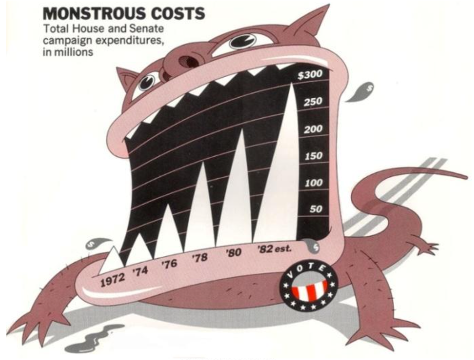
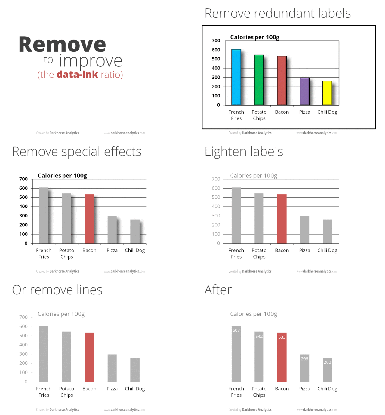
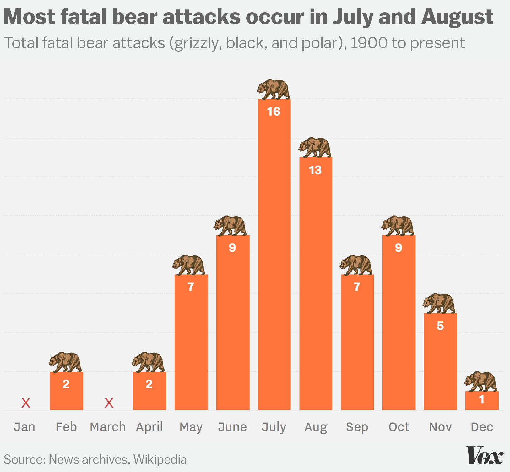
“Erase non-data ink.”

— Ed Tufte

Figure 1.6: `Monstrous Costs’ by Nigel Holmes, in Healy, 2018

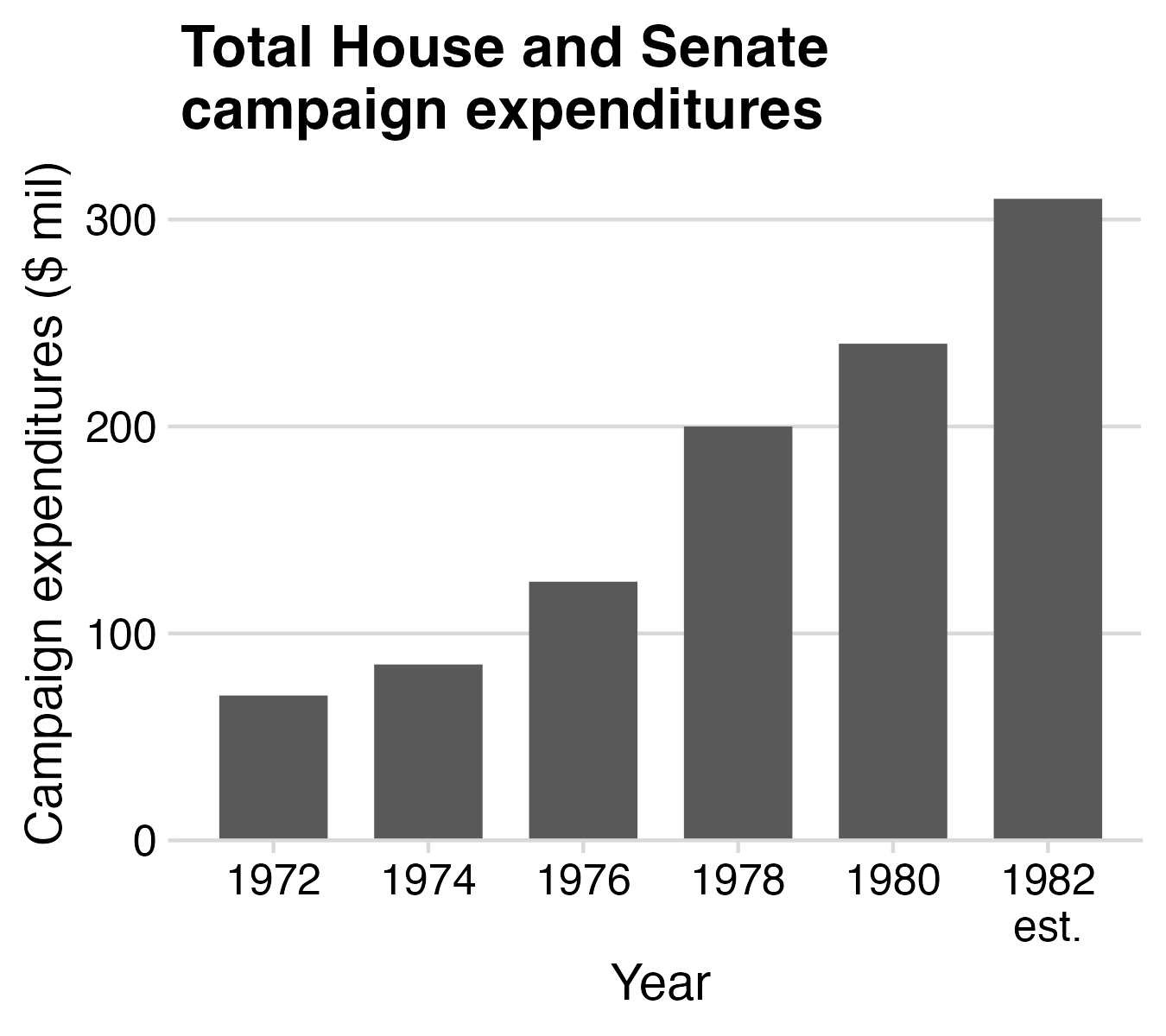
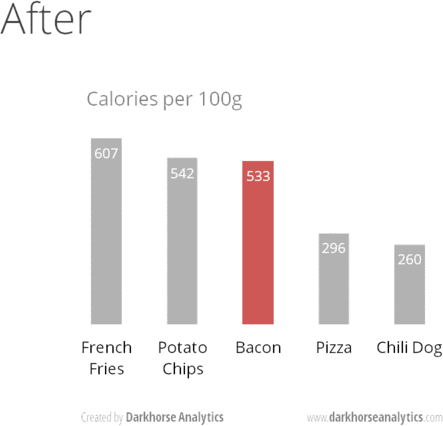
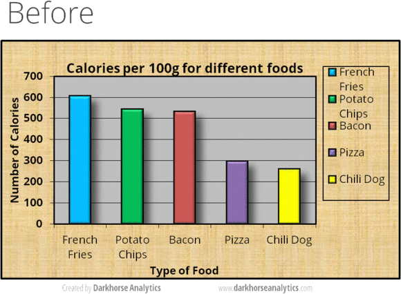
Figure 24.1: From Data Looks Better Naked by Darkhorse Analytics

10 Data Viz Best Practices

1. Remove chart chunk
2. Don’t make 3D plots*
3. Don’t lie
4. Don’t use pie charts for proportions*
5. Don’t stack bars*
6. Rotate and sort categorical axes*
7. Eliminate legends & directly label geoms*
8. Don’t use pattern fills
9. Don’t use red & green together
10. Consider tables for small data sets

*most of the time

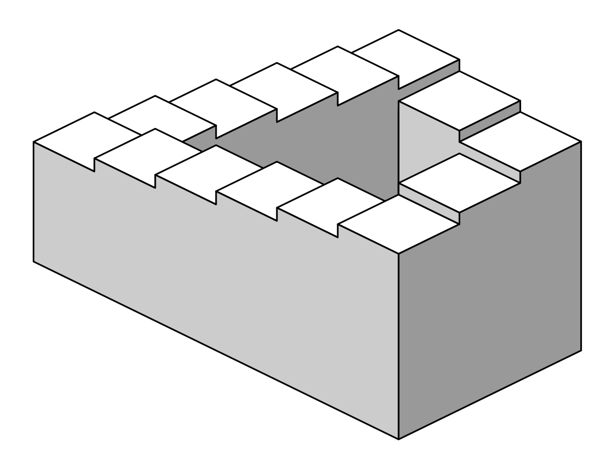
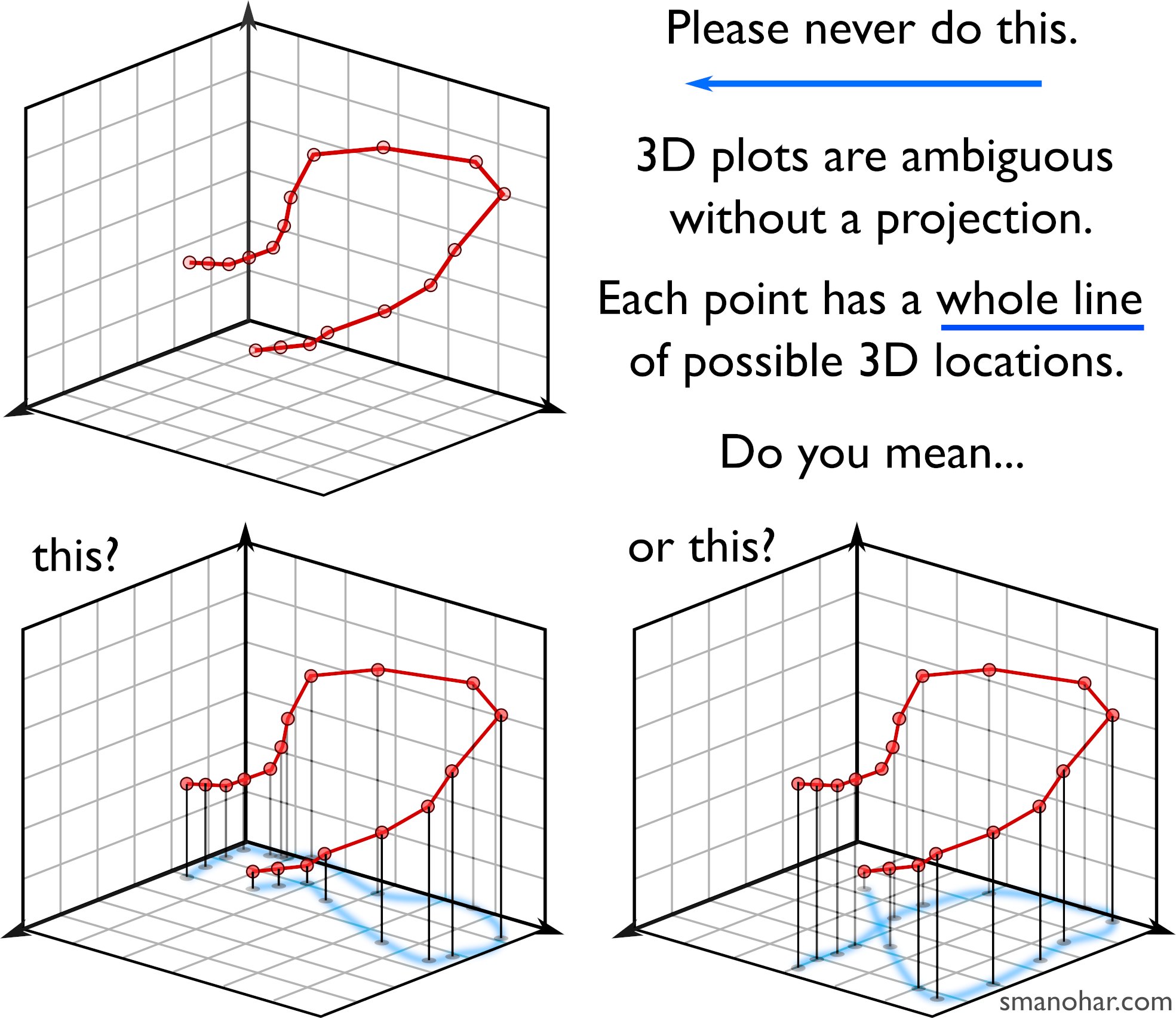
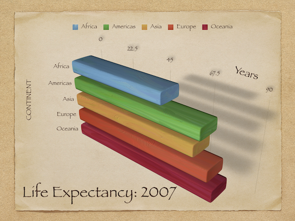
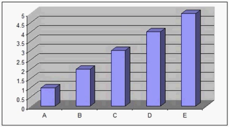
Humans aren’t good at distinguishing 3D space

Penrose Stairs, made famous by
M.C. Escher (1898-1972)

Ink proportions !=
true proportions

Occlusion: geoms are obscured

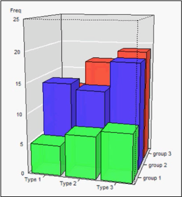
Multiple interpretations

The third dimension distracts from the data

(this is what Tufte calls “chart junk”)

10 Data Viz Best Practices

1. Remove chart chunk
2. Don’t make 3D plots*
3. Don’t lie
4. Don’t use pie charts for proportions*
5. Don’t stack bars*
6. Rotate and sort categorical axes*
7. Eliminate legends & directly label geoms*
8. Don’t use pattern fills
9. Don’t use red & green together
10. Consider tables for small data sets

*most of the time

Edward Tufte (2001) “The Visual Display of Quantitative Information”, 2nd Edition, pg. 57-58.

Bar charts should always start at 0

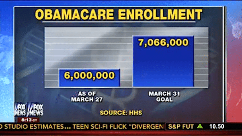
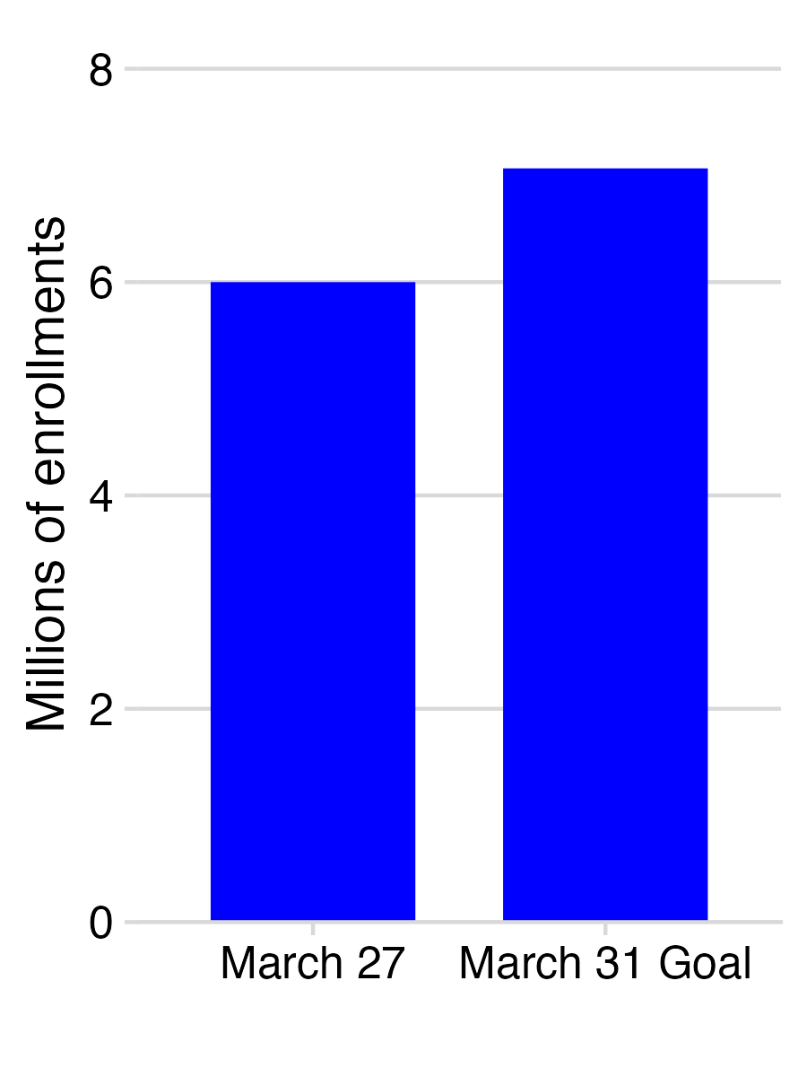
Bar charts should always start at 0

Image from http://livingqlikview.com/the-9-worst-data-visualizations-ever-created/

Don’t cherry-pick your data

Don’t cherry-pick your data

Image from https://www.mediamatters.org/fox-news/fox-news-newest-dishonest-chart-immigration-enforcement

Make sure your chart makes sense

Image from http://livingqlikview.com/the-9-worst-data-visualizations-ever-created/

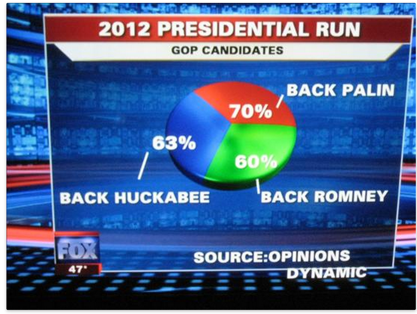
10 Data Viz Best Practices

1. Remove chart chunk
2. Don’t make 3D plots*
3. Don’t lie
4. Don’t use pie charts for proportions*
5. Don’t stack bars*
6. Rotate and sort categorical axes*
7. Eliminate legends & directly label geoms*
8. Don’t use pattern fills
9. Don’t use red & green together
10. Consider tables for small data sets

*most of the time

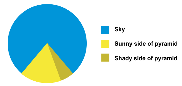
Exceptions:

- Small data

- Simple fractions

- If sum of parts matters

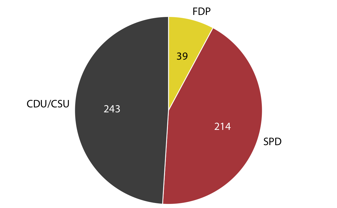
Best pie chart of all time

10 Data Viz Best Practices

1. Remove chart chunk
2. Don’t make 3D plots*
3. Don’t lie
4. Don’t use pie charts for proportions*
5. Don’t stack bars*
6. Rotate and sort categorical axes*
7. Eliminate legends & directly label geoms*
8. Don’t use pattern fills
9. Don’t use red & green together
10. Consider tables for small data sets

*most of the time

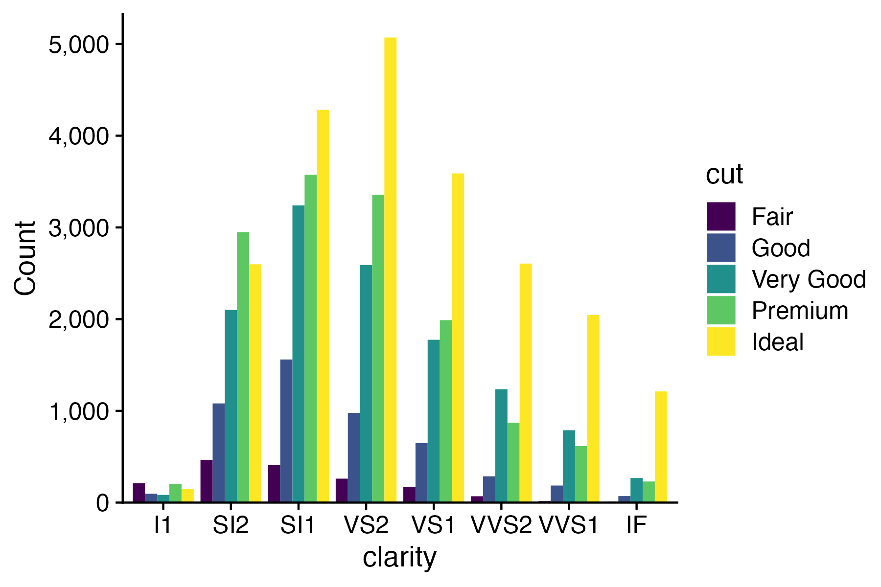
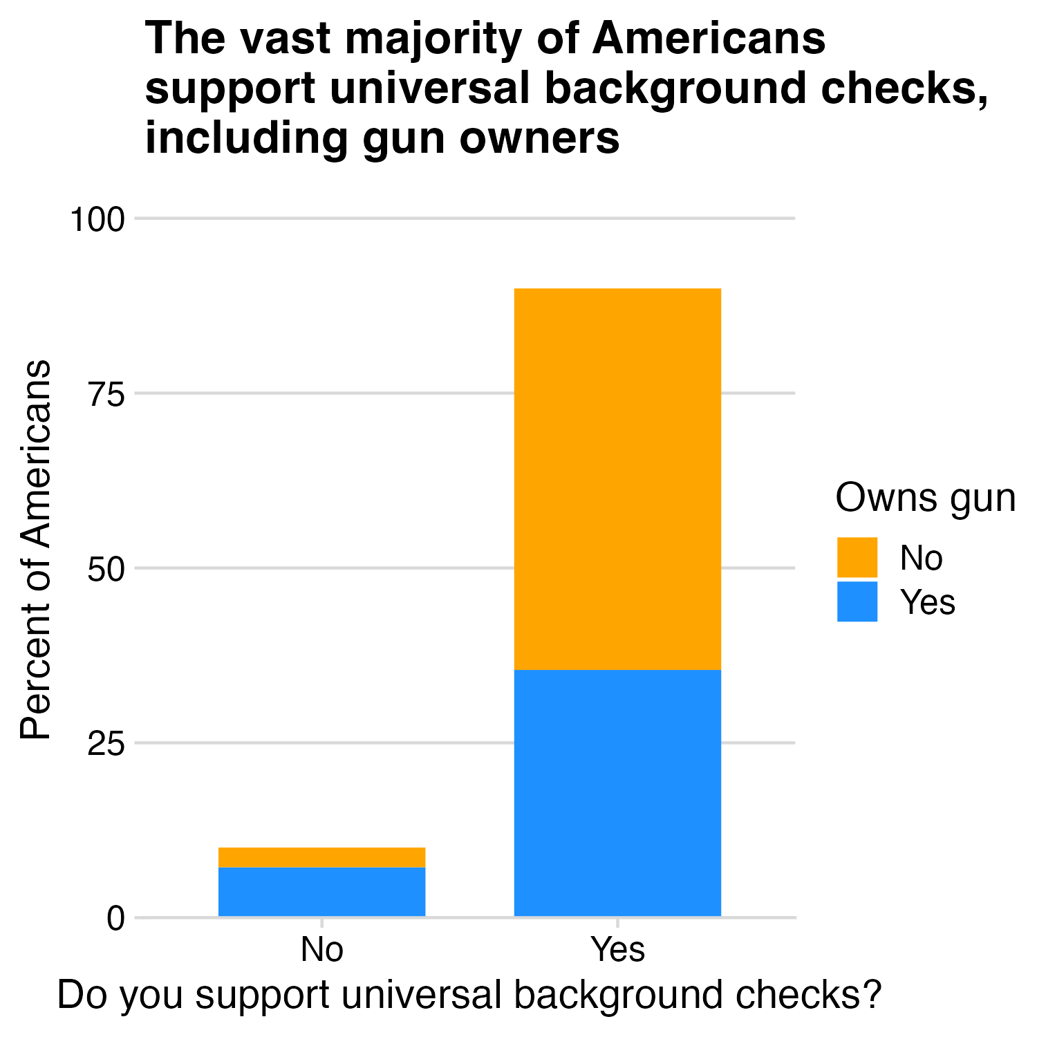
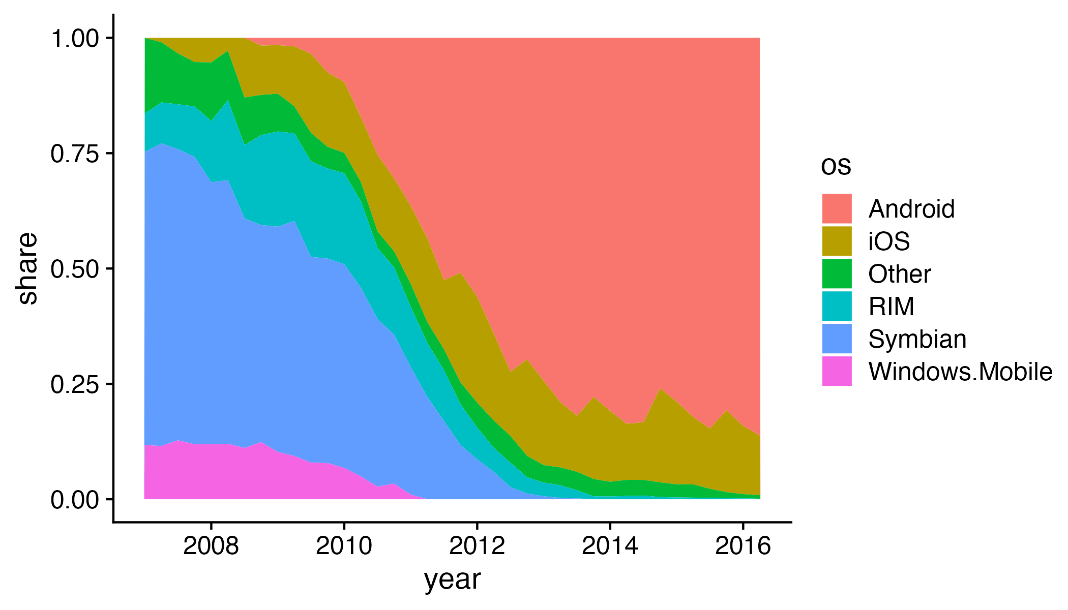
Stacked bars are rarely a good idea

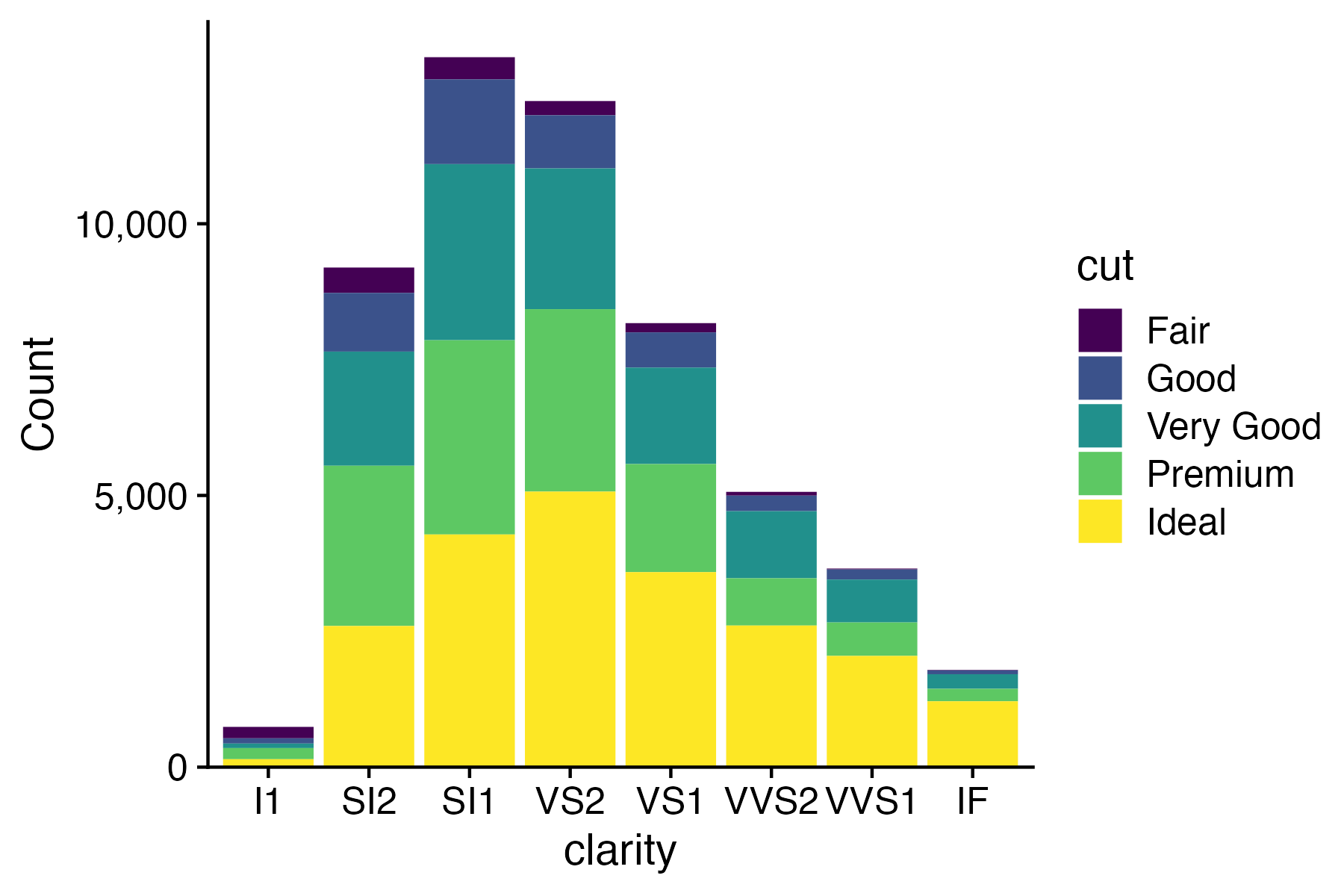
“Parallel coordinates” plot usually works better

Exception:
When you care about the total more than the categories

10 Data Viz Best Practices

1. Remove chart chunk
2. Don’t make 3D plots*
3. Don’t lie
4. Don’t use pie charts for proportions*
5. Don’t stack bars*
6. Rotate and sort categorical axes*
7. Eliminate legends & directly label geoms*
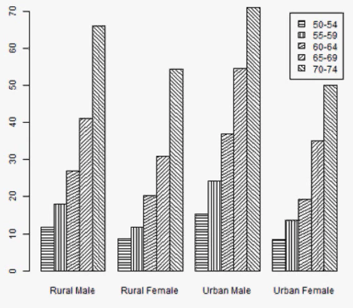
8. Don’t use pattern fills
9. Don’t use red & green together
10. Consider tables for small data sets

*most of the time

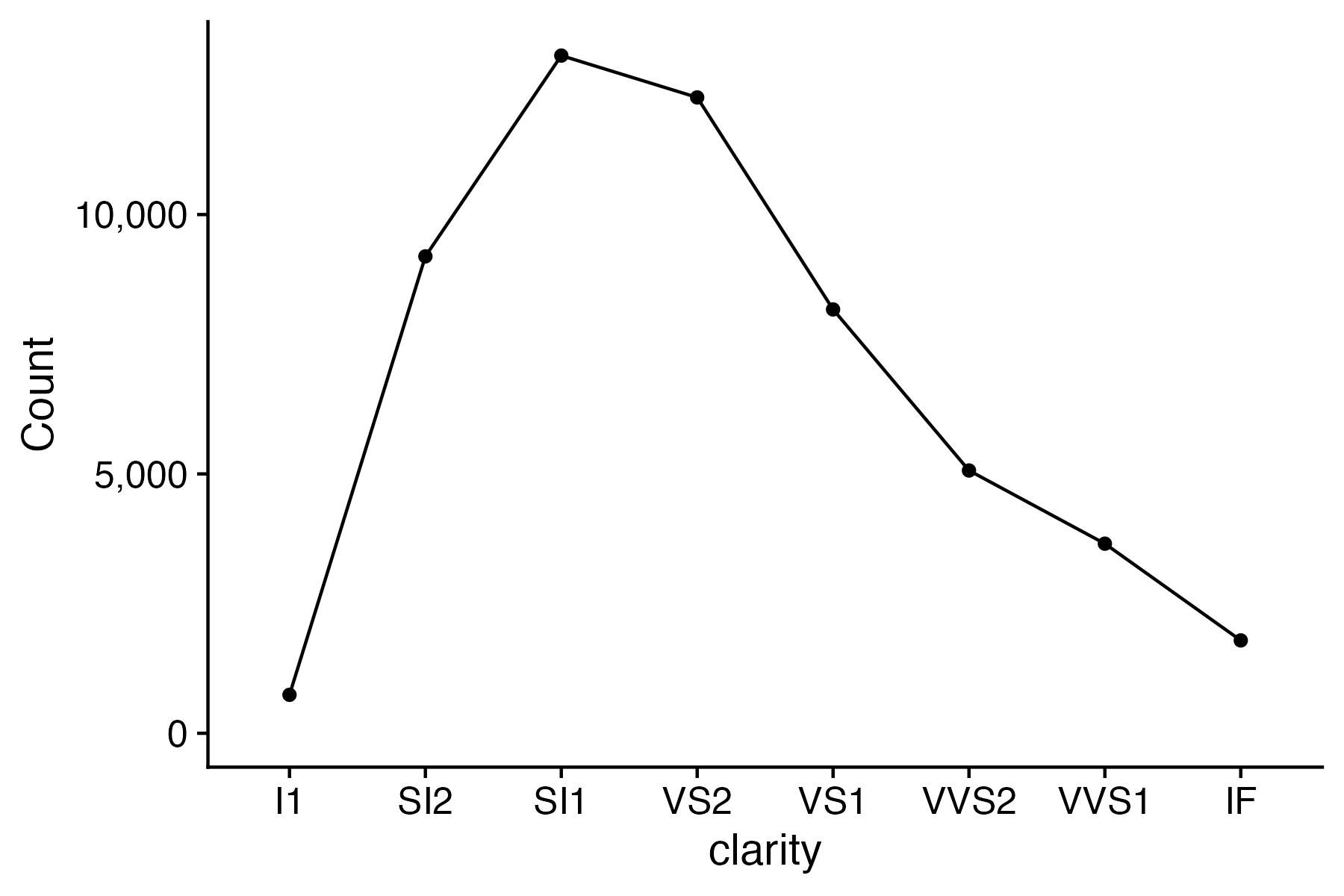
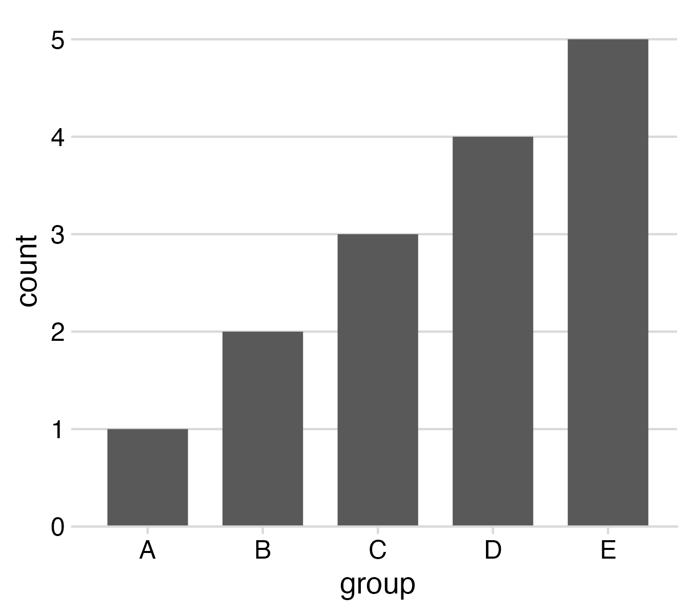
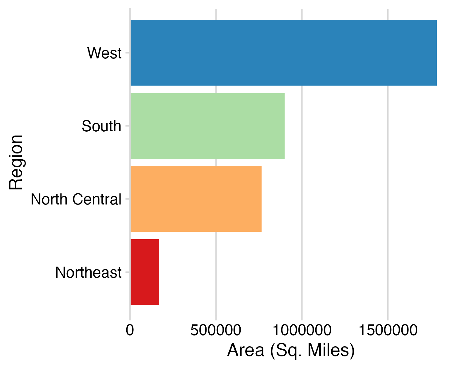
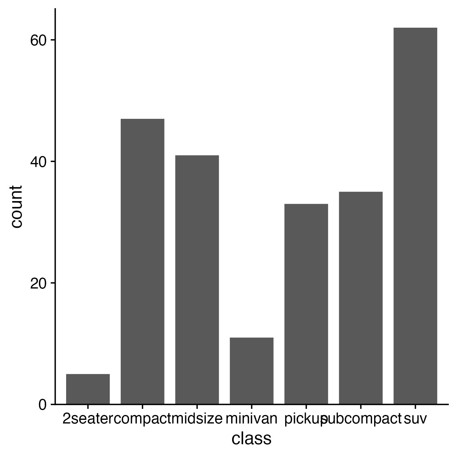
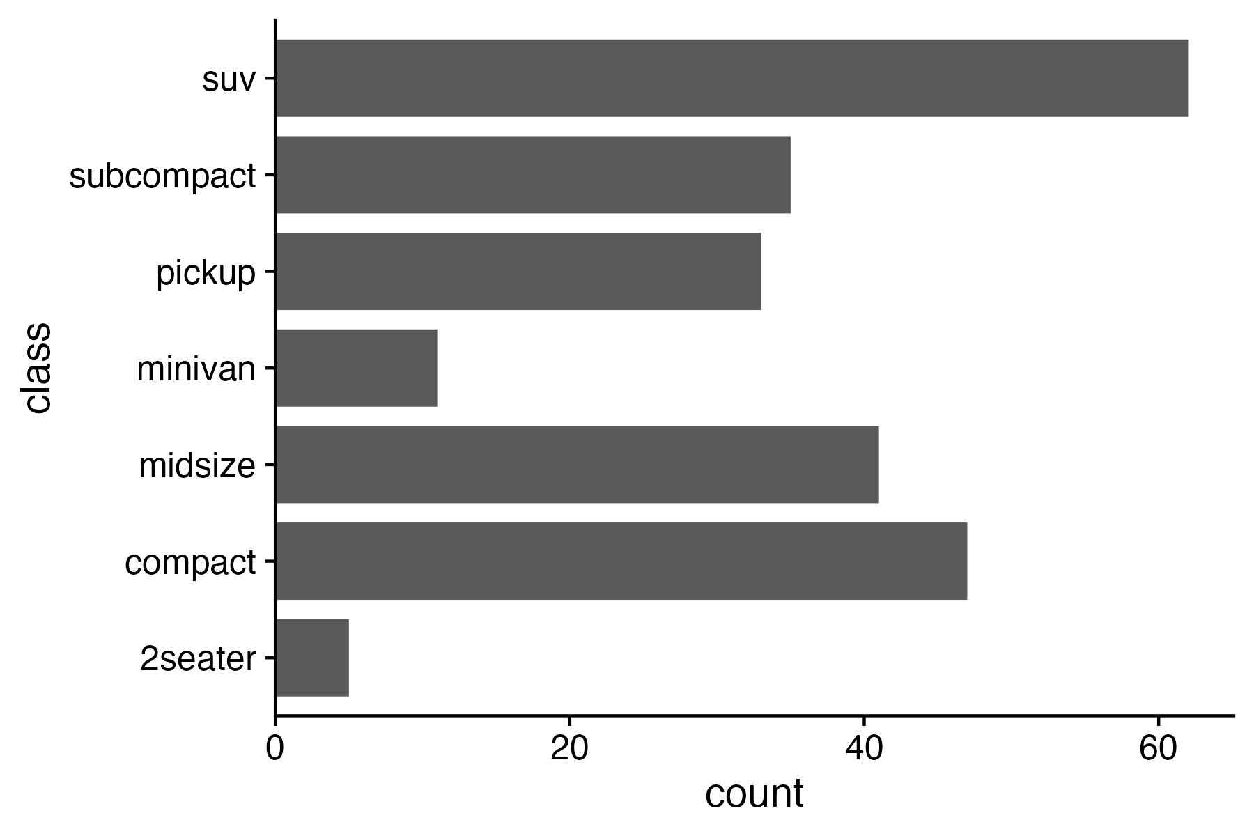
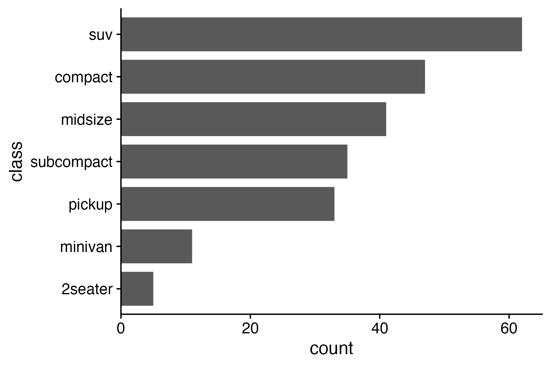
Rotate axes if you can’t read them

Default order is almost always wrong

Ordered by alphabet (default)

Ordered by count

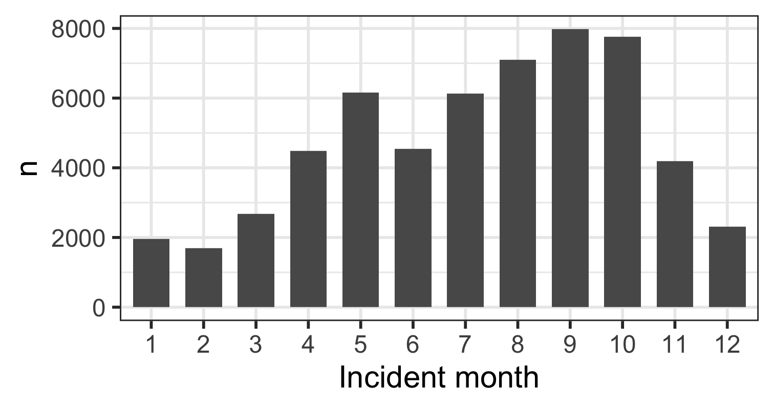
Exception: Ordinal variables

10 Data Viz Best Practices

1. Remove chart chunk
2. Don’t make 3D plots*
3. Don’t lie
4. Don’t use pie charts for proportions*
5. Don’t stack bars*
6. Rotate and sort categorical axes*
7. Eliminate legends & directly label geoms*
8. Don’t use pattern fills
9. Don’t use red & green together
10. Consider tables for small data sets

*most of the time

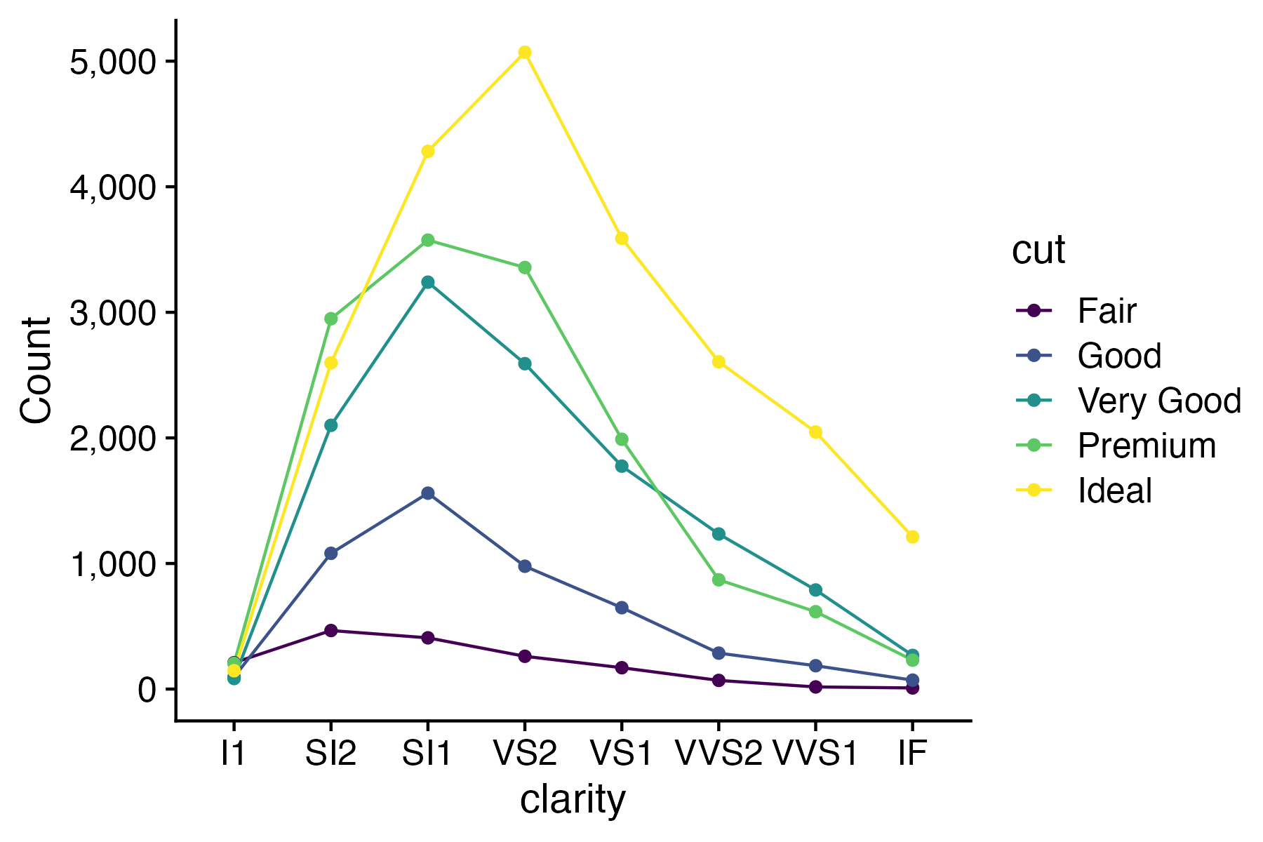
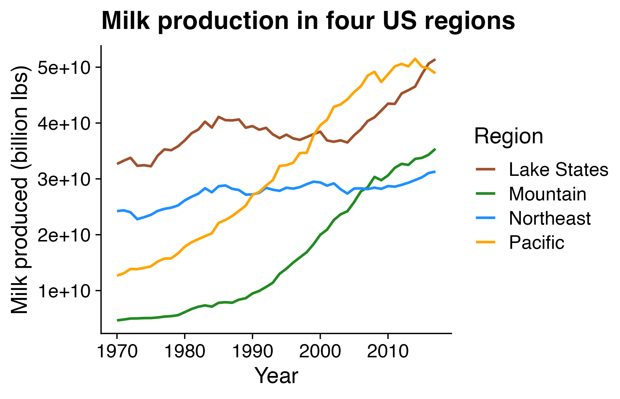
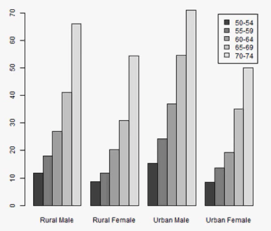
Directly label geoms

Exception: When you have repeated categories

10 Data Viz Best Practices

1. Remove chart chunk
2. Don’t make 3D plots*
3. Don’t lie
4. Don’t use pie charts for proportions*
5. Don’t stack bars*
6. Rotate and sort categorical axes*
7. Eliminate legends & directly label geoms*
8. Don’t use pattern fills
9. Don’t use red & green together
10. Consider tables for small data sets

*most of the time

10 Data Viz Best Practices

1. Remove chart chunk
2. Don’t make 3D plots*
3. Don’t lie
4. Don’t use pie charts for proportions*
5. Don’t stack bars*
6. Rotate and sort categorical axes*
7. Eliminate legends & directly label geoms*
8. Don’t use pattern fills
9. Don’t use red & green together
10. Consider tables for small data sets

*most of the time

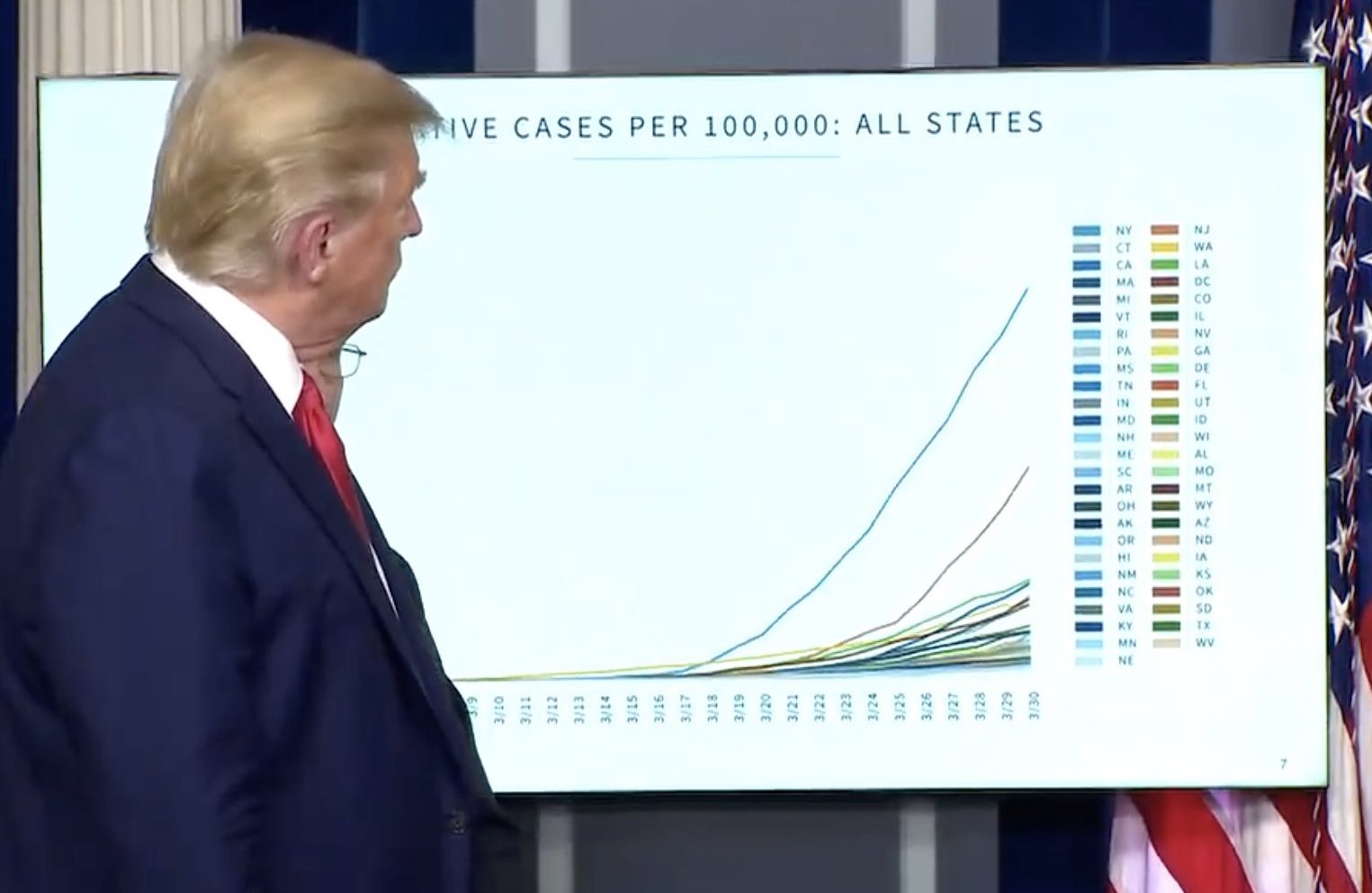
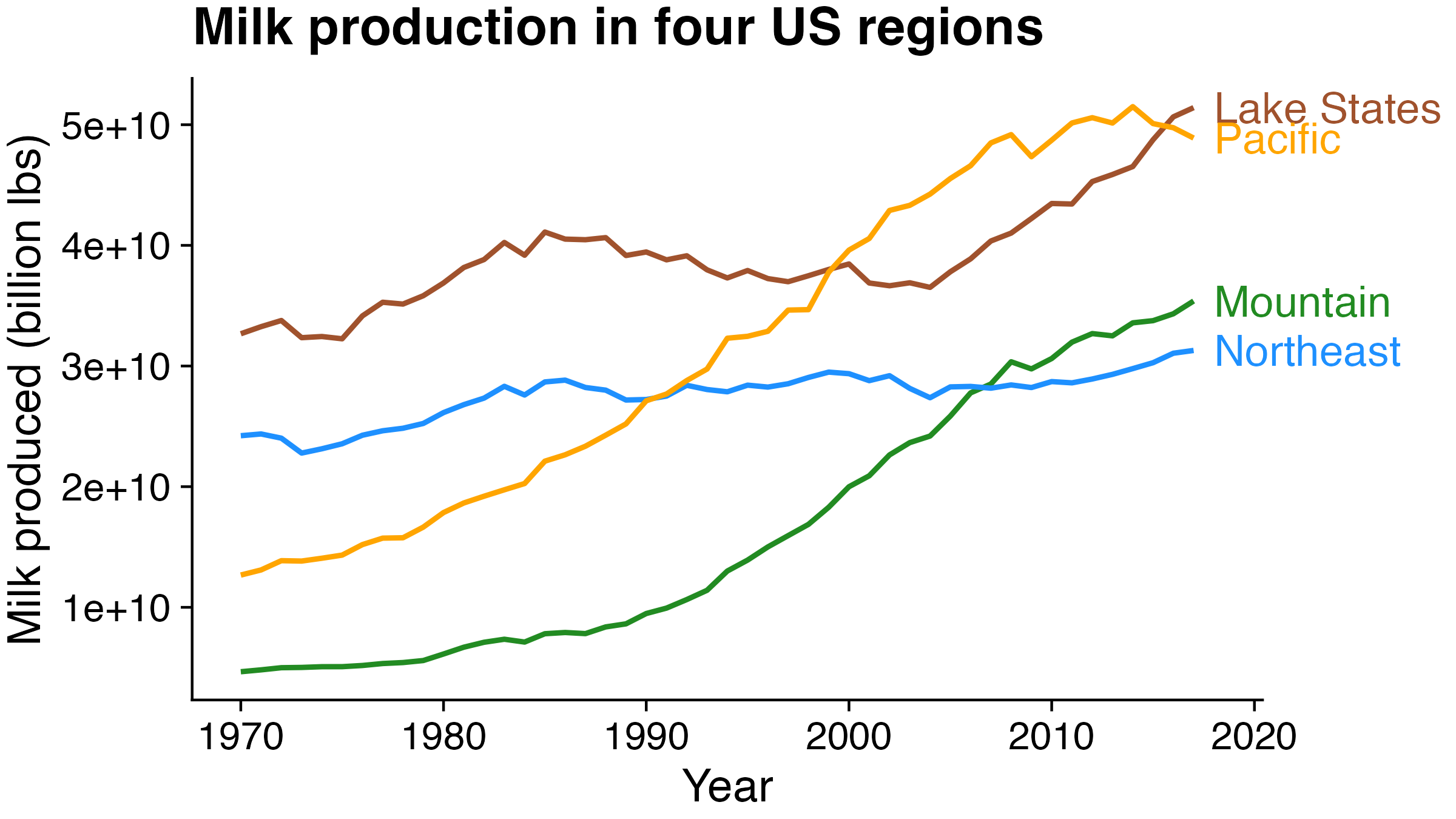
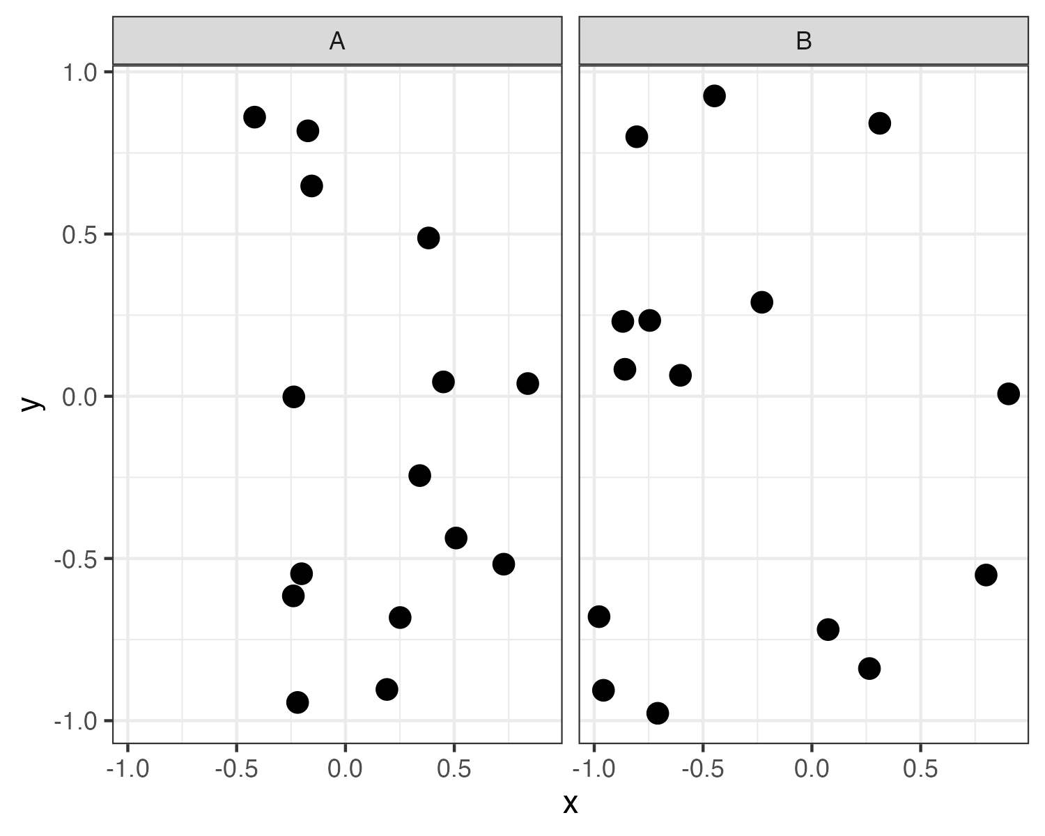
10% of males and 1% of females are color blind

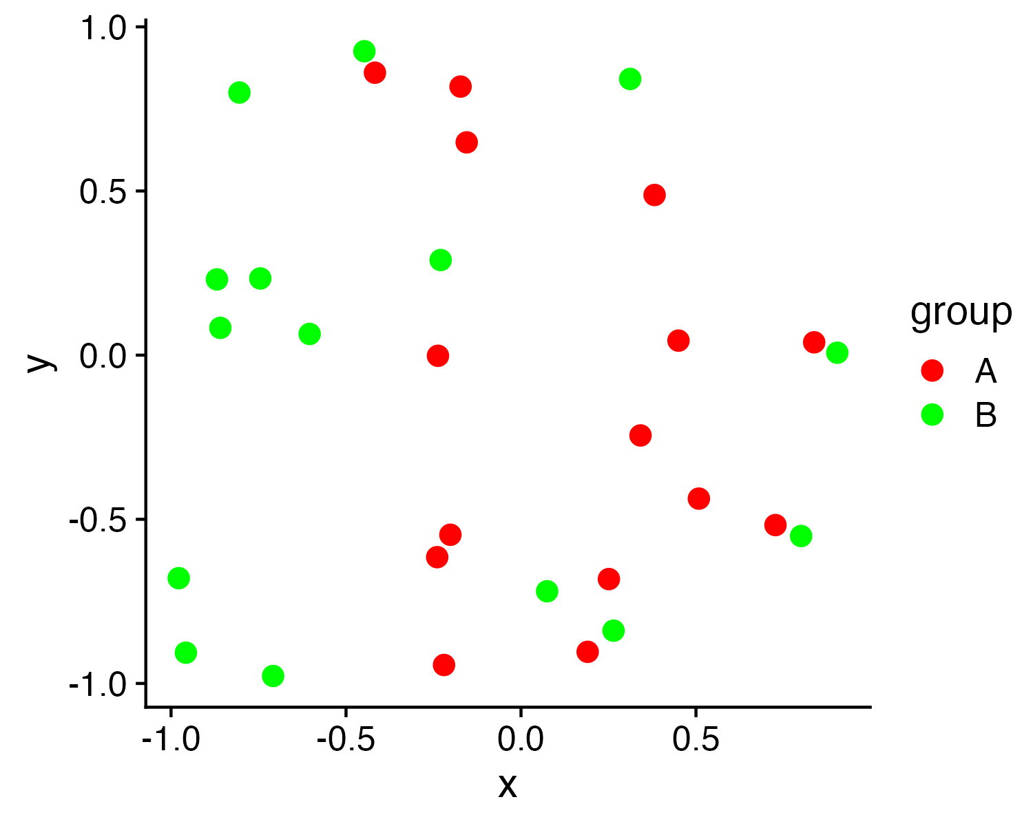
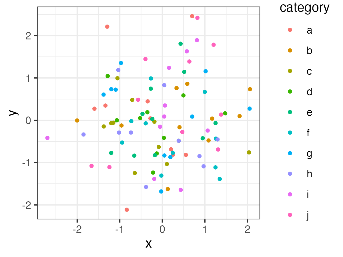
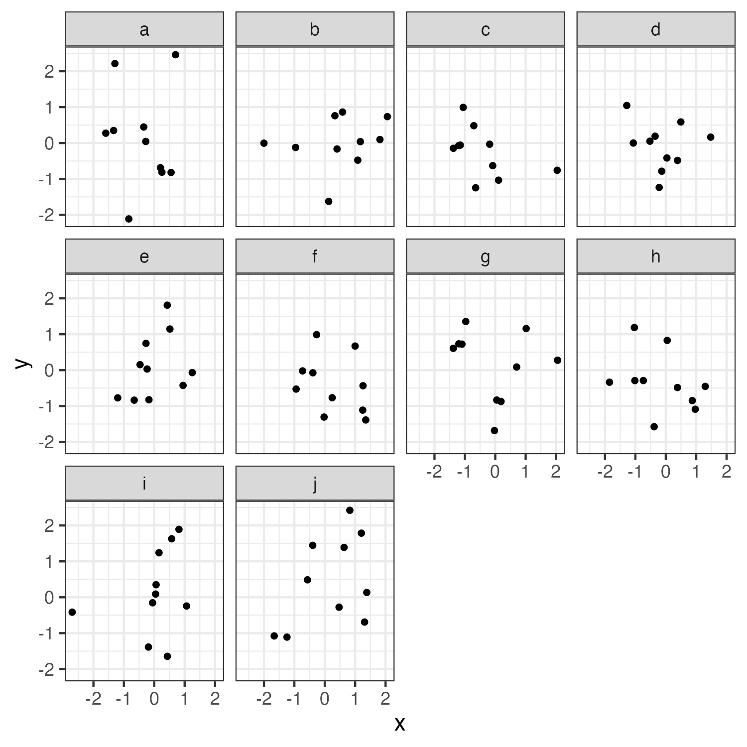
Facets can be used to avoid color altogether

10 Data Viz Best Practices

1. Remove chart chunk
2. Don’t make 3D plots*
3. Don’t lie
4. Don’t use pie charts for proportions*
5. Don’t stack bars*
6. Rotate and sort categorical axes*
7. Eliminate legends & directly label geoms*
8. Don’t use pattern fills
9. Don’t use red & green together
10. Consider tables for small data sets

*most of the time

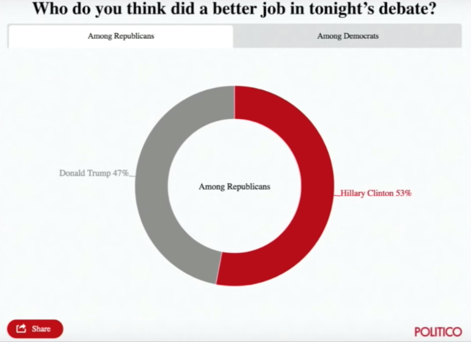
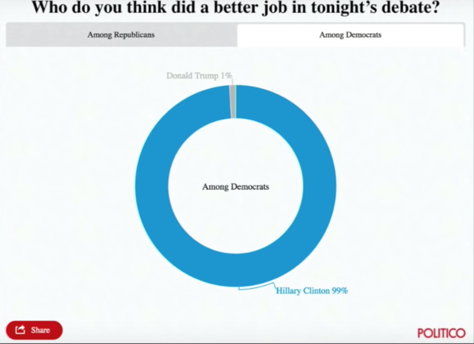
Who do you think did a better job in tonight’s debate?

	Clinton	Trump
Among Democrats	99%	1%
Among Republicans	53%	47%

References:

- Data Viz “Cheat Sheet”

- Data Viz Reference Page

Your turn - go here

For your “bad” visualization:

1. Identify where the graphic falls on Cleveland’s pattern recognition hierarchy

2. Any design rules that are broken

3. Suggest at least two improvements

10:00

Week 7: Visualizing Information

1. The Human Visual-Memory System

2. The Psychology of Data Viz

3. 10 Data Viz Best Practices

4. Making a (good) ggplot

Making a (good) ggplot

Before:

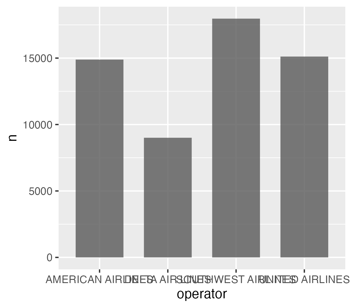
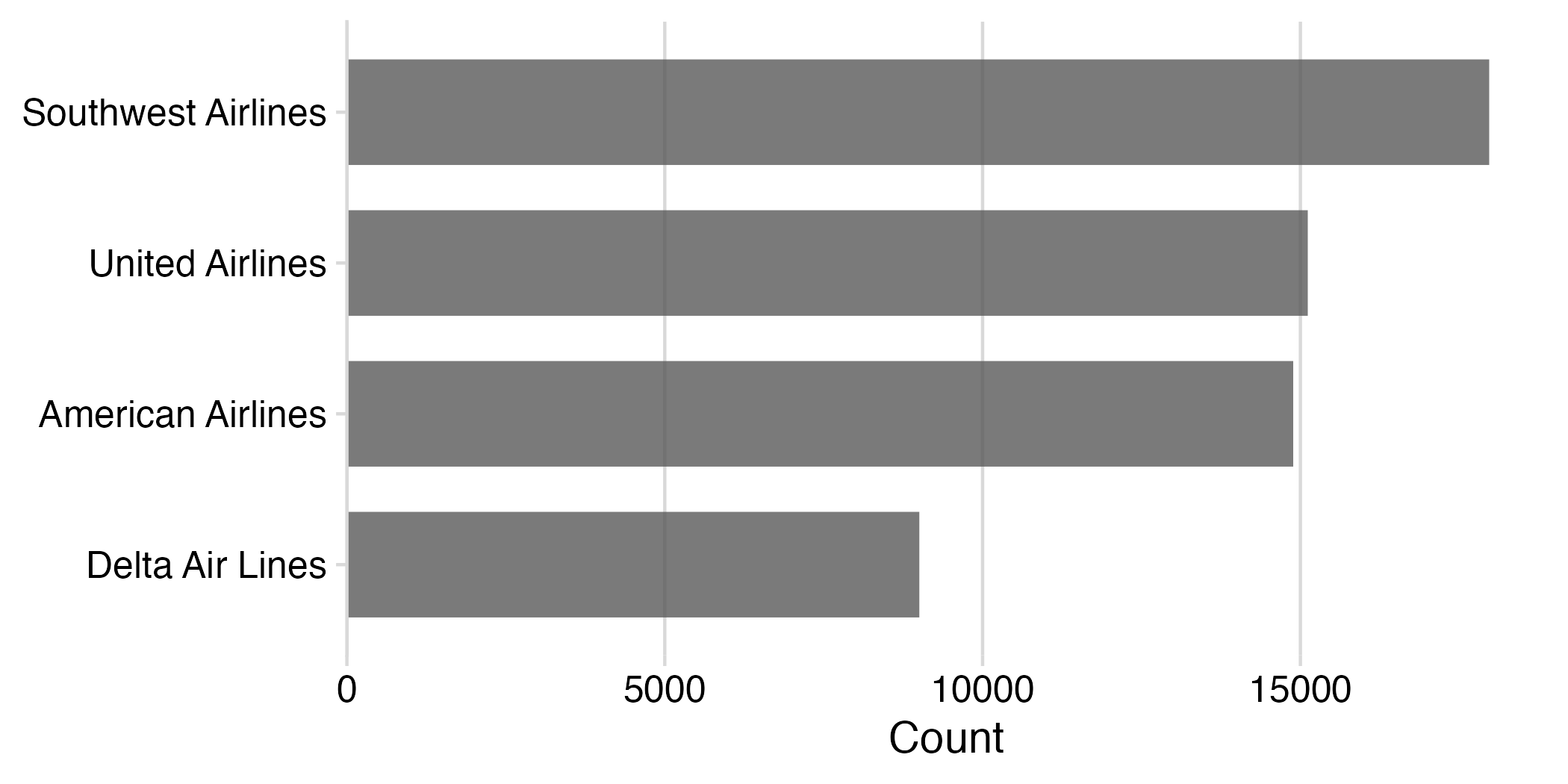
After:

Making a (good) ggplot

1. Format data frame
2. Add geoms
3. Flip coordinates?
4. Reorder factors?
5. Adjust scales
6. Adjust theme
7. Annotate

1) Format data frame

# Format the data frame
wildlife_impacts %>%
  count(operator)

#> # A tibble: 4 × 2
#>   operator               n
#>   <chr>              <int>
#> 1 AMERICAN AIRLINES  14887
#> 2 DELTA AIR LINES     9005
#> 3 SOUTHWEST AIRLINES 17970
#> 4 UNITED AIRLINES    15116

2) Add geoms

# Format the data frame
wildlife_impacts %>%
  count(operator) %>%

  # Add geoms
  ggplot() +
  geom_col(
    aes(x = operator, y = n),
    width = 0.7,
    alpha = 0.8
  )

3) Flip coordinates - can you read the labels?

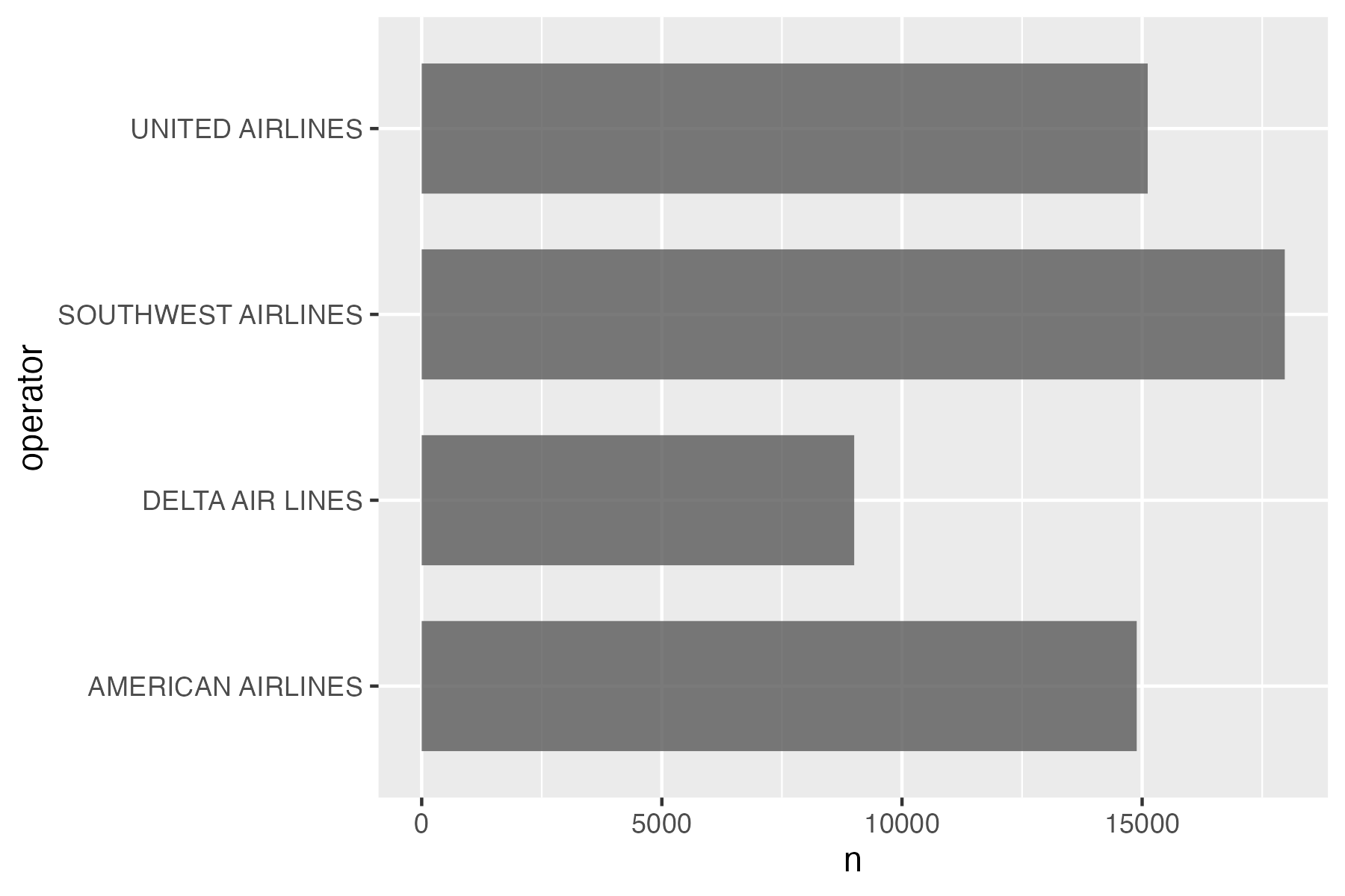
# Format the data frame
wildlife_impacts %>%
  count(operator) %>%

  # Add geoms
  ggplot() +
  geom_col(
    aes(x = operator, y = n),
    width = 0.7,
    alpha = 0.8
  ) +

  # Flip coordinates
  coord_flip()

3) Flip coordinates - can you read the labels?

# Format the data frame
wildlife_impacts %>%
  count(operator) %>%

  # Add geoms
  ggplot() +
  geom_col(
    aes(x = n, y = operator),
    width = 0.7,
    alpha = 0.8
  )

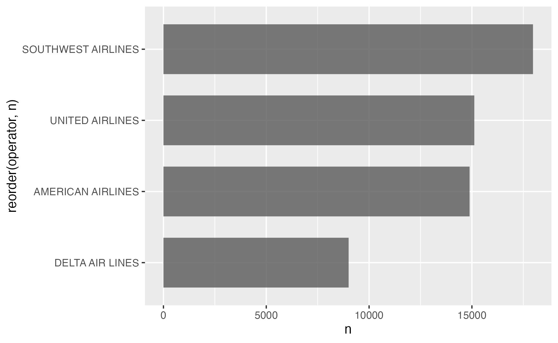
4) Reorder factors with reorder()

# Format the data frame
wildlife_impacts %>%
  count(operator) %>%

  # Add geoms
  ggplot() +
  geom_col(
    aes(x = n, y = reorder(operator, n)),
    width = 0.7,
    alpha = 0.8
  )

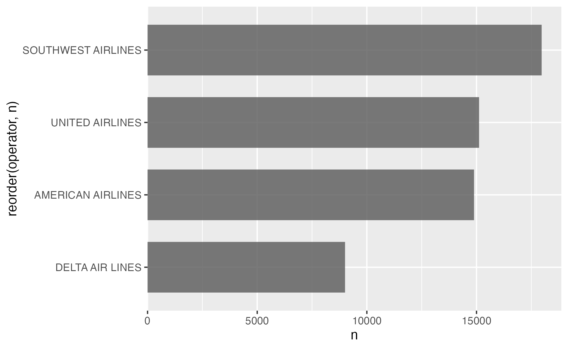
5) Adjust scales

# Format the data frame
wildlife_impacts %>%
  count(operator) %>%

  # Add geoms
  ggplot() +
  geom_col(
    aes(x = n, y = reorder(operator, n)),
    width = 0.7,
    alpha = 0.8
  ) +

  # Adjust x axis scale
  scale_x_continuous(
    expand = expansion(mult = c(0, 0.05))
  )

5) Adjust scales - customize break points (if you want)

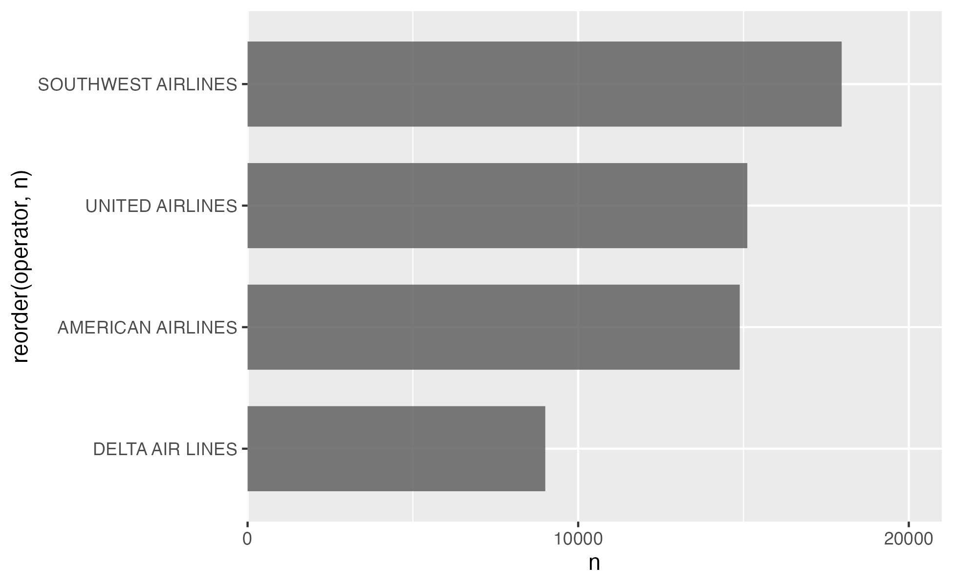
# Format the data frame
wildlife_impacts %>%
  count(operator) %>%

  # Add geoms
  ggplot() +
  geom_col(
    aes(x = n, y = reorder(operator, n)),
    width = 0.7,
    alpha = 0.8
  ) +

  # Adjust x axis scale
  scale_x_continuous(
    expand = expansion(mult = c(0, 0.05)),
    breaks = c(0, 10000, 20000),
    limits = c(0, 20000)
  )

6) Adjust theme

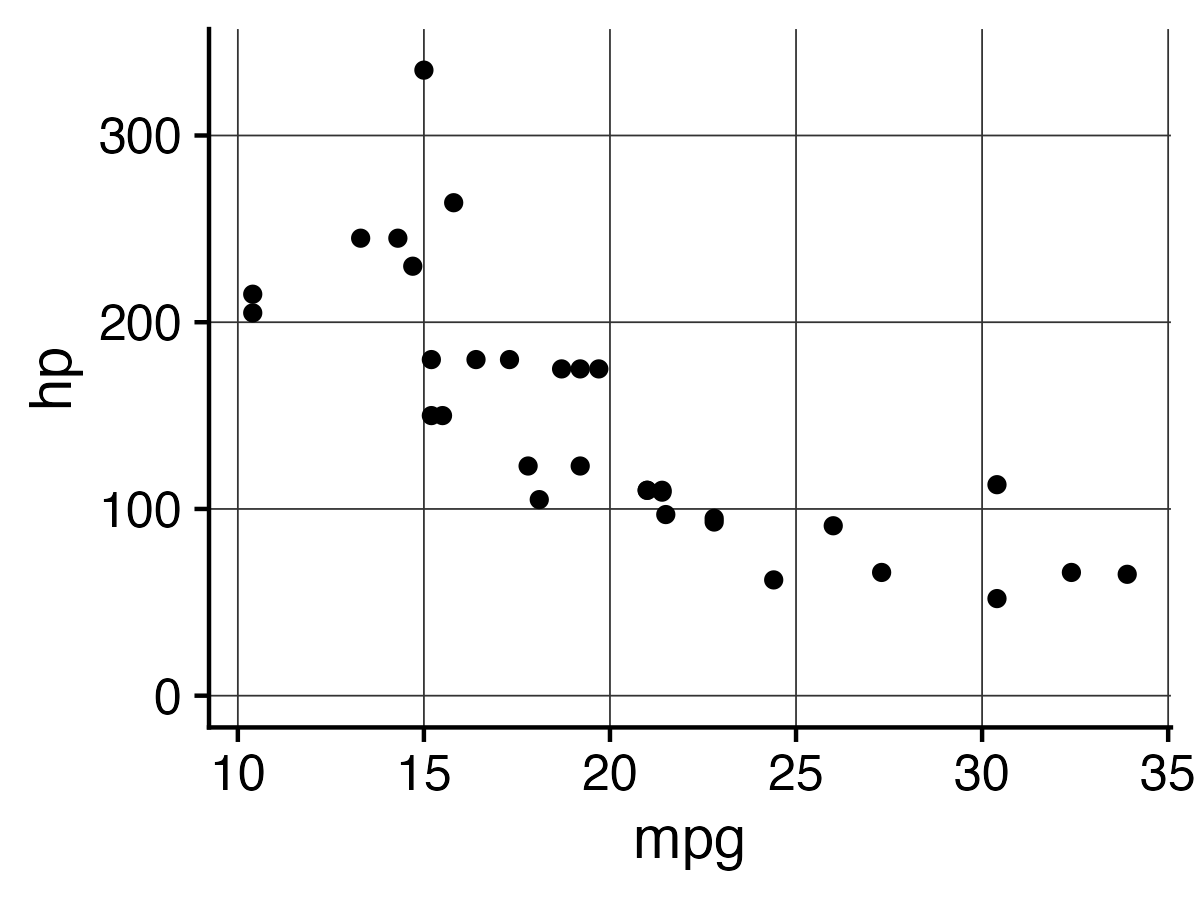
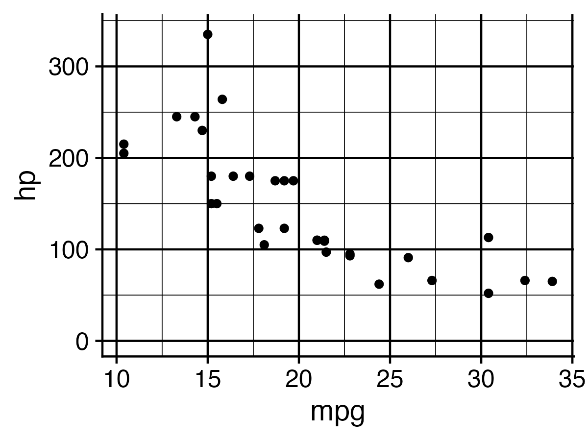
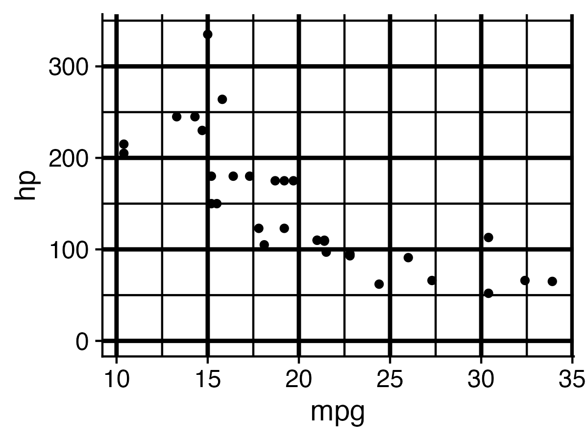
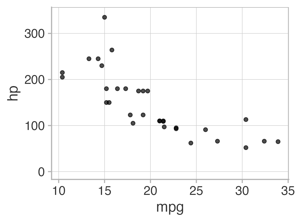
Four cowplot themes you should know

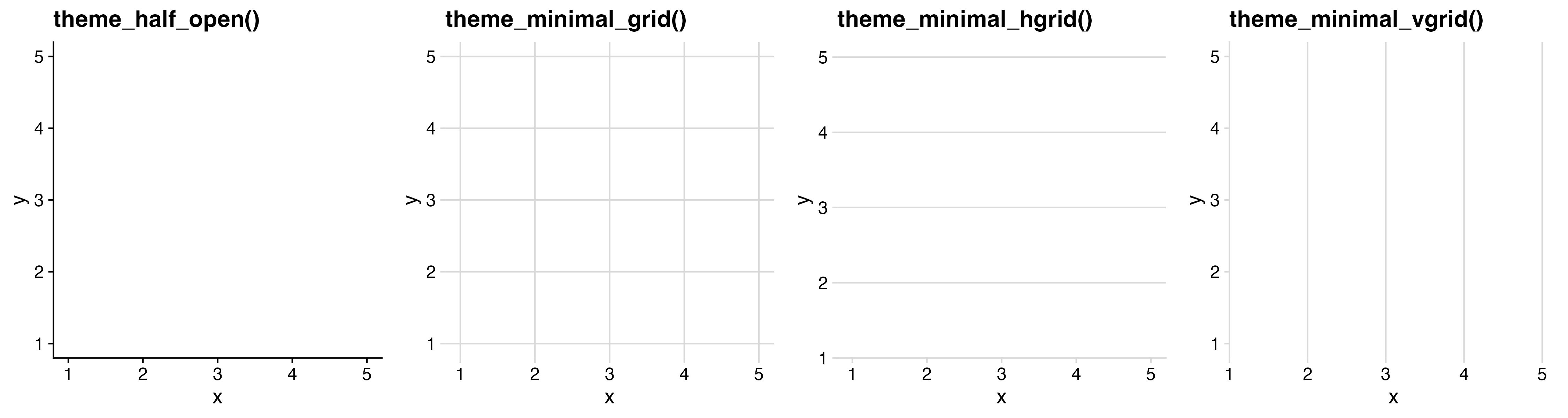
6) Adjust theme

For horizontal bars, add only vertical grid

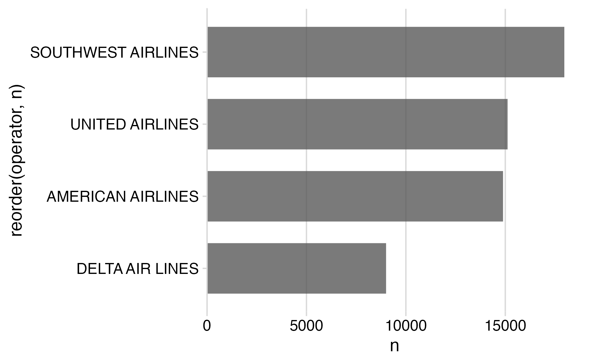
# Format the data frame
wildlife_impacts %>%
  count(operator) %>%

  # Add geoms
  ggplot() +
  geom_col(
    aes(x = n, y = reorder(operator, n)),
    width = 0.7,
    alpha = 0.8
  ) +

  # Adjust x axis scale
  scale_x_continuous(
    expand = expansion(mult = c(0, 0.05))
  ) +

  # Adjust theme
  theme_minimal_vgrid()

7) Annotate

# Format the data frame
wildlife_impacts %>%
  count(operator) %>%
  mutate(operator = str_to_title(operator)) %>%

  # Add geoms
  ggplot() +
  geom_col(
    aes(x = n, y = reorder(operator, n)),
    width = 0.7,
    alpha = 0.8
  ) +

  # Adjust x axis scale
  scale_x_continuous(
    expand = expansion(mult = c(0, 0.05))
  ) +

  # Adjust theme
  theme_minimal_vgrid() +

  # Annotate
  labs(
    x = 'Count',
    y = NULL
  )

Finished product

wildlife_impacts %>%
  count(operator) %>%
  mutate(operator = str_to_title(operator)) %>%
  ggplot() +
  geom_col(
    aes(x = n, y = reorder(operator, n)),
    width = 0.7,
    alpha = 0.8
  ) +
  scale_x_continuous(
    expand = expansion(mult = c(0, 0.05))
  ) +
  theme_minimal_vgrid() +
  labs(
    x = 'Count',
    y = NULL
  )

15:00

Your turn

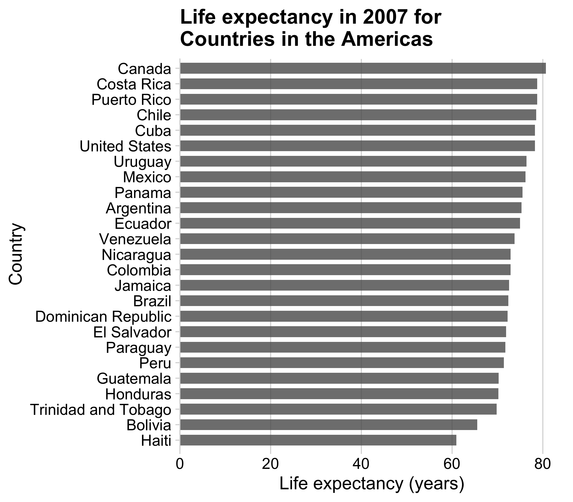
Use the gapminder.csv data to create the following plot, following these steps:

1. Format data frame
2. Add geoms
3. Flip coordinates?
4. Reorder factors?
5. Adjust scales
6. Adjust theme
7. Annotate