Factors, Amounts, & Proportions

EMSE 4572/6572: Exploratory Data Analysis

John Paul Helveston

October 14, 2026

Quiz 3

Write your name on the quiz!

Rules:

Work alone; no outside help of any kind is allowed.
No calculators, no notes, no books, no computers, no phones.

Next projects due:

- Mini project 2: Exploring Data (Due 10/25)

- Initial Report (Due 11/01)

Today’s data

avengers <- read_csv(file.path('data', 'avengers.csv'))
bears <- read_csv(file.path('data', 'north_america_bear_killings.csv'))
federal_spending <- read_csv(file.path('data', 'fed_spend_long.csv'))
gapminder <- read_csv(file.path('data', 'gapminder.csv'))
lotr_words <- read_csv(file.path('data', 'lotr_words.csv'))
milk_production <- read_csv(file.path('data', 'milk_production.csv'))
wildlife_impacts <- read_csv(file.path('data', 'wildlife_impacts.csv'))

New packages

The {waffle} package

install.packages("waffle")

Week 8: Factors, Amounts, & Proportions

1. Manipulating factors

2. Graphing amounts

3. Graphing proportions

Week 8: Factors, Amounts, & Proportions

1. Manipulating factors

2. Graphing amounts

3. Graphing proportions

Sorting in ggplot is done by reordering factors

Two ways to sort

Method 1: Use reorder() inside aesthetic mapping

# Format the data frame
federal_spending %>%
  group_by(department) %>%
  summarise(
    rd_budget_bil = sum(rd_budget_mil) / 10^3
  ) %>%

  # Make the chart
  ggplot() +
  geom_col(
    aes(
      x = rd_budget_bil,
      y = reorder(department, rd_budget_bil)
    ),
    width = 0.7,
    alpha = 0.8,
    fill = "steelblue"
  ) +
  scale_x_continuous(
    expand = expansion(mult = c(0, 0.05))
  ) +
  theme_minimal_vgrid()

Two ways to sort

Method 2: Use fct_reorder() when formatting the data frame

# Format the data frame
federal_spending %>%
  group_by(department) %>%
  summarise(
    rd_budget_bil = sum(rd_budget_mil) / 10^3
  ) %>%
  mutate(
    department = fct_reorder(department, rd_budget_bil)
  ) %>%
  # Make the chart
  ggplot() +
  geom_col(
    aes(x = rd_budget_bil, y = department),
    width = 0.7,
    alpha = 0.8,
    fill = "steelblue"
  ) +
  scale_x_continuous(
    expand = expansion(mult = c(0, 0.05))
  ) +
  theme_minimal_vgrid()

Reorder & modify factors with
the forcats library

Loaded with library(tidyverse)

Common situations for modifying / reording factors:

1. Reorder factors based on another numerical variable

2. Reorder factors manually

3. Modify factors manually

4. What if there are too many factor levels?

1. Reorder factors based on another numerical variable

Use fct_reorder()

# Format the data frame
federal_spending %>%
  group_by(department) %>%
  summarise(
    rd_budget_bil = sum(rd_budget_mil) / 10^3
  ) %>%
  mutate(
    department = fct_reorder(department, rd_budget_bil)
  ) %>%
  # Make the chart
  ggplot() +
  geom_col(
    aes(x = rd_budget_bil, y = department),
    width = 0.7,
    alpha = 0.8,
    fill = "steelblue"
  ) +
  scale_x_continuous(
    expand = expansion(mult = c(0, 0.05))
  ) +
  theme_minimal_vgrid()

2. Reorder factors manually

# Format the data frame
lotr_words %>%
  pivot_longer(
    names_to = 'gender',
    values_to = 'wordCount',
    cols = Female:Male
  ) %>%

  # Make the chart
  ggplot() +
  geom_col(
    aes(x = wordCount, y = Film),
    width = 0.7,
    alpha = 0.8
  ) +
  scale_x_continuous(
    expand = expansion(mult = c(0, 0.05))
  ) +
  theme_minimal_vgrid()

2. Reorder factors manually with `fct_relevel()`

# Format the data frame
lotr_words %>%
  pivot_longer(
    names_to = 'gender',
    values_to = 'wordCount',
    cols = Female:Male
  ) %>%
  mutate(
    Film = fct_relevel(
      Film,
      levels = c(
        'The Fellowship Of The Ring',
        'The Two Towers',
        'The Return Of The King'
      )
    )
  ) %>%

  # Make the chart
  ggplot() +
  geom_col(
    aes(x = wordCount, y = Film),
    width = 0.7,
    alpha = 0.8
  ) +
  scale_x_continuous(
    expand = expansion(mult = c(0, 0.05))
  ) +
  theme_minimal_vgrid()

3. Modify factors manually

# Format the data frame
lotr_words %>%
  pivot_longer(
    names_to = 'gender',
    values_to = 'wordCount',
    cols = Female:Male
  ) %>%

  # Make the chart
  ggplot() +
  geom_col(
    aes(x = wordCount, y = Film),
    width = 0.7,
    alpha = 0.8
  ) +
  scale_x_continuous(
    expand = expansion(mult = c(0, 0.05))
  ) +
  theme_minimal_vgrid()

The film names here are too long

3. Modify factors manually with `fct_recode()`

"new label" = "old label"

# Format the data frame
lotr_words %>%
  pivot_longer(
    names_to = 'gender',
    values_to = 'wordCount',
    cols = Female:Male
  ) %>%
  mutate(
    Film = fct_recode(
      Film,
      'The Fellowship\nof the Ring' = 'The Fellowship Of The Ring',
      'The Return\nof the King' = 'The Return Of The King'
    )
  ) %>%

  # Make the chart
  ggplot() +
  geom_col(
    aes(x = wordCount, y = Film),
    width = 0.7,
    alpha = 0.8
  ) +
  scale_x_continuous(
    expand = expansion(mult = c(0, 0.05))
  ) +
  theme_minimal_vgrid()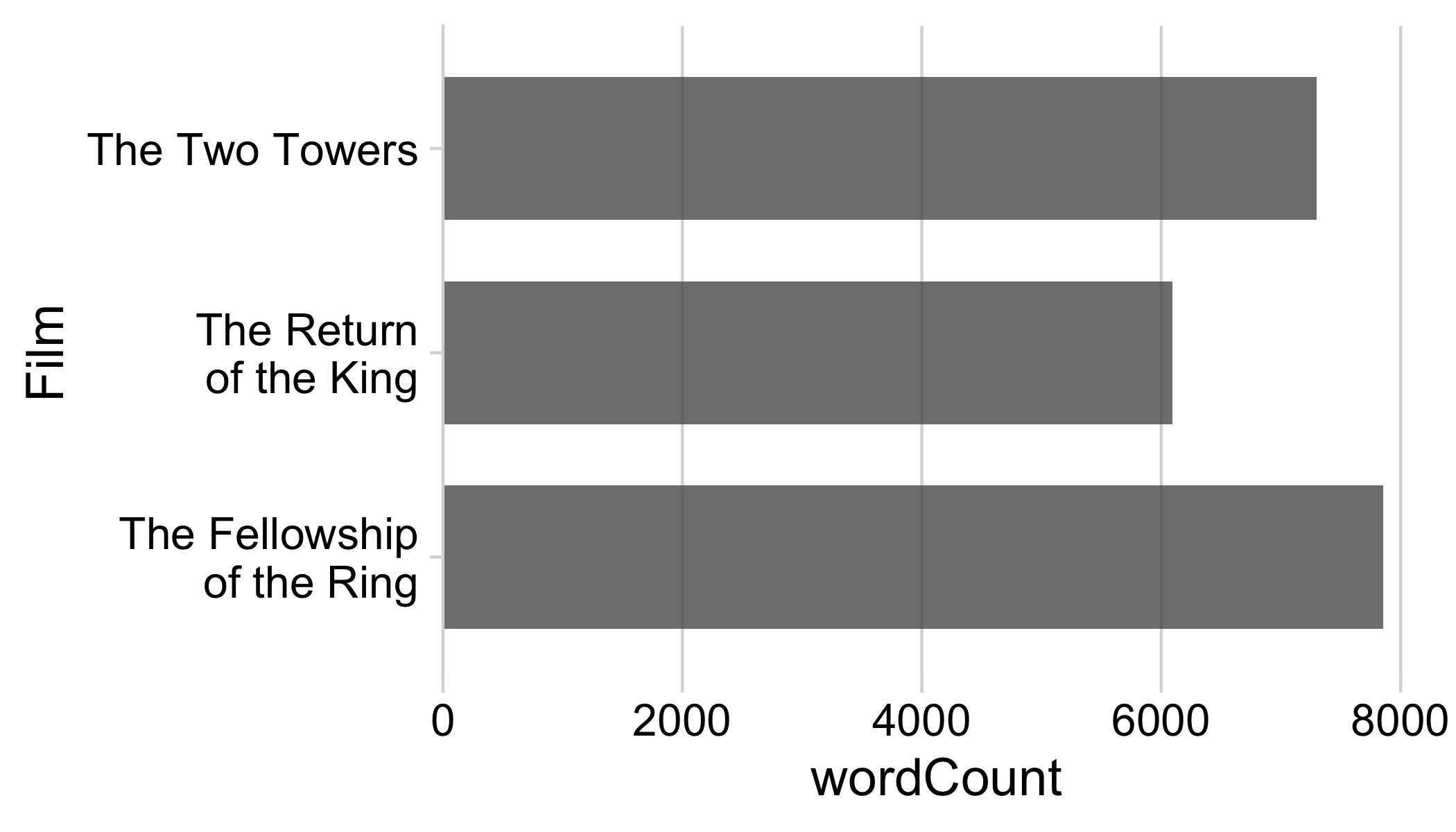

2 & 3. Modify and reorder factors manually

# Format the data frame
lotr_words %>%
  pivot_longer(
    names_to = 'gender',
    values_to = 'wordCount',
    cols = Female:Male
  ) %>%
  mutate(
    Film = fct_relevel(
      Film,
      levels = c(
        'The Fellowship Of The Ring',
        'The Two Towers',
        'The Return Of The King'
      )
    ),
    Film = fct_recode(
      Film,
      'The Fellowship\nof the Ring' = 'The Fellowship Of The Ring',
      'The Return\nof the King' = 'The Return Of The King'
    )
  ) %>%

  # Make the chart
  ggplot() +
  geom_col(
    aes(x = wordCount, y = Film),
    width = 0.7,
    alpha = 0.8
  ) +
  scale_x_continuous(expand = expansion(mult = c(0, 0.05))) +
  theme_minimal_vgrid()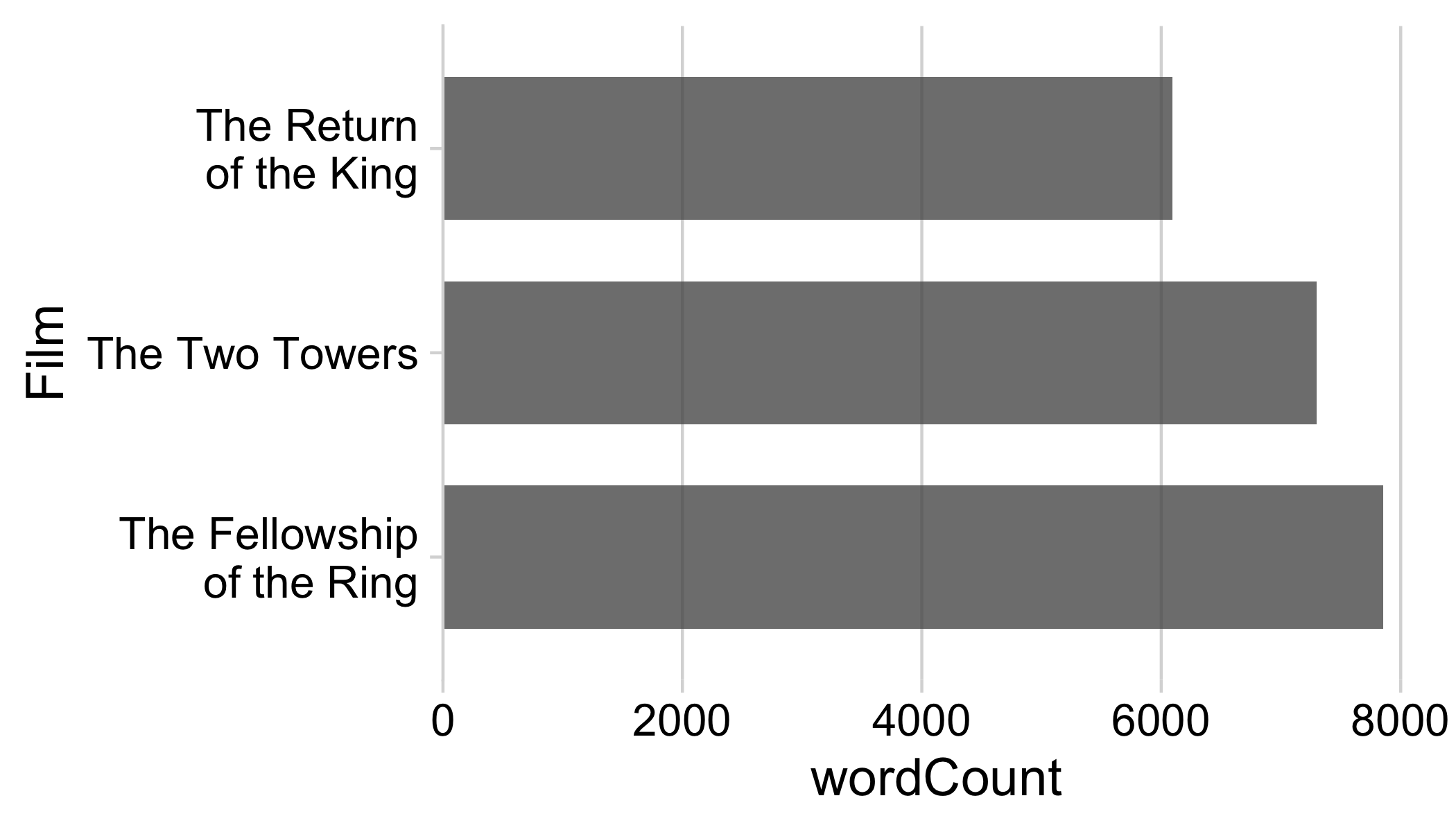

4. What if there are too many factor levels?

# Format the data frame
federal_spending %>%
  group_by(department) %>%
  summarise(
    rd_budget_bil = sum(rd_budget_mil) / 10^3
  ) %>%
  mutate(
    department = fct_reorder(department, rd_budget_bil)
  ) %>%
  # Make the chart
  ggplot() +
  geom_col(
    aes(x = rd_budget_bil, y = department),
    width = 0.7,
    alpha = 0.8,
    fill = "steelblue"
  ) +
  scale_x_continuous(
    expand = expansion(mult = c(0, 0.05))
  ) +
  theme_minimal_vgrid()

4. What if there are too many factor levels?

Strategy: Merge smaller factors into “Other” with fct_other()

# Format the data frame
federal_spending %>%
  mutate(
    department = fct_other(
      department,
      keep = c('DOD', 'HHS', 'NIH', 'NASA', 'DOE')
    )
  ) %>%
  group_by(department) %>%
  summarise(
    rd_budget_bil = sum(rd_budget_mil) / 10^3
  ) %>%
  mutate(
    department = fct_reorder(department, rd_budget_bil)
  ) %>%

  # Make the chart
  ggplot() +
  geom_col(
    aes(x = rd_budget_bil, y = department),
    width = 0.7,
    alpha = 0.8,
    fill = "steelblue"
  ) +
  scale_x_continuous(
    expand = expansion(mult = c(0, 0.05))
  ) +
  theme_minimal_vgrid()

4. What if there are really too many factor levels?

# Format the data frame
avengers %>%
  mutate(
    name_alias = fct_reorder(name_alias, appearances)
  ) %>%

  # Make the chart
  ggplot() +
  geom_col(
    aes(x = appearances, y = name_alias),
    width = 0.7,
    alpha = 0.8
  ) +
  scale_x_continuous(
    expand = expansion(mult = c(0, 0.05))
  ) +
  theme_minimal_vgrid()

4. What if there are really too many factor levels?

Strategy: Keep top N, drop the rest with slice()

# Format the data frame
avengers %>%
  mutate(
    name_alias = fct_reorder(name_alias, appearances)
  ) %>%
  arrange(desc(appearances)) %>%
  slice(1:10) %>%

  # Make the chart
  ggplot() +
  geom_col(
    aes(x = appearances, y = name_alias),
    width = 0.7,
    alpha = 0.8
  ) +
  scale_x_continuous(
    expand = expansion(mult = c(0, 0.05))
  ) +
  theme_minimal_vgrid()

4. What if there are really too many factor levels?

slice() works with grouping too!

# Format the data frame
avengers %>%
  mutate(
    name_alias = fct_reorder(name_alias, appearances)
  ) %>%
  arrange(desc(appearances)) %>%
  group_by(gender) %>%
  slice(1:10) %>%

  # Make the chart
  ggplot() +
  geom_col(
    aes(
      x = appearances,
      y = name_alias,
      fill = gender
    ),
    width = 0.7,
    alpha = 0.8
  ) +
  scale_x_continuous(
    expand = expansion(mult = c(0, 0.05))
  ) +
  theme_minimal_vgrid()

Your turn - practice manipulating factors

Use the wildlife_impacts data to create the following plot

Week 8: Factors, Amounts, & Proportions

1. Manipulating factors

2. Graphing amounts

3. Graphing proportions

Show amounts with:

Bar chart

Dot chart

Lollipop chart

Bars are good for highlighting specific categories

Use lollipops when:

- The bars are overwhelming
- You’re not highlighting categories

Or use dots and don’t set axis to 0

How to make a Bar chart

# Summarize the data
federal_spending %>%
  group_by(department) %>%
  summarise(rd_budget_bil = sum(rd_budget_mil) / 10^3) %>%
  mutate(department = fct_reorder(department, rd_budget_bil)) %>%

  # Make chart
  ggplot() +
  geom_col(
    aes(x = rd_budget_bil, y = department),
    width = 0.7,
    alpha = 0.8,
    fill = 'steelblue'
  ) +
  scale_x_continuous(
    expand = expansion(mult = c(0, 0.05))
  ) +
  theme_minimal_vgrid()

Filling the bars with color

# Summarize the data
federal_spending %>%
  group_by(department) %>%
  summarise(rd_budget_bil = sum(rd_budget_mil) / 10^3) %>%
  mutate(
    department = fct_reorder(department, rd_budget_bil),
    is_dod = if_else(department == 'DOD', TRUE, FALSE)
  ) %>%

  # Make the chart
  ggplot() +
  geom_col(
    aes(x = rd_budget_bil, y = department, fill = is_dod),
    width = 0.7,
    alpha = 0.8
  ) +
  scale_x_continuous(
    expand = expansion(mult = c(0, 0.05))
  ) +
  theme_minimal_vgrid() +
  theme(legend.position = 'none')

The DOD’s R&D budget is nearly the same as all other departments combined

Filling the bars with color

# Summarize the data
federal_spending %>%
  group_by(department) %>%
  summarise(rd_budget_bil = sum(rd_budget_mil) / 10^3) %>%
  mutate(
    department = fct_reorder(department, rd_budget_bil),
    is_dod = if_else(
      department == 'DOD',
      TRUE,
      FALSE
    )
  ) %>%

  # Make the chart
  ggplot() +
  geom_col(
    aes(x = rd_budget_bil, y = department, fill = is_dod),
    width = 0.7,
    alpha = 0.8
  ) +
  scale_x_continuous(expand = expansion(mult = c(0, 0.05))) +
  scale_fill_manual(values = c('grey', 'steelblue')) +
  theme_minimal_vgrid() +
  theme(legend.position = 'none')

The DOD’s R&D budget is nearly the same as all other departments combined

How to make a Dot chart

Summarize data frame:

# Summarize the data
federal_spending %>%
  group_by(department) %>%
  summarise(
    rd_budget_bil = sum(rd_budget_mil) / 10^3
  ) %>%
  mutate(
    department = fct_reorder(department, rd_budget_bil)
  ) %>%

  # Make the chart
  ggplot() +
  geom_point(
    aes(x = rd_budget_bil, y = department),
    size = 2.5,
    color = 'steelblue'
  ) +
  theme_minimal_vgrid()

Dot chart of federal R&D spending by department

How to make a Lollipop chart

Summarize data frame:

# Summarize the data
federal_spending %>%
  group_by(department) %>%
  summarise(
    rd_budget_bil = sum(rd_budget_mil) / 10^3
  ) %>%
  mutate(
    department = fct_reorder(department, rd_budget_bil)
  ) %>%

  # Make the chart
  ggplot() +
  geom_segment(
    aes(x = 0, xend = rd_budget_bil, y = department, yend = department),
    color = 'grey'
  ) +
  geom_point(
    aes(x = rd_budget_bil, y = department),
    size = 2.5,
    color = 'steelblue'
  ) +
  theme_minimal_vgrid()

Lollipop chart of federal R&D spending by department

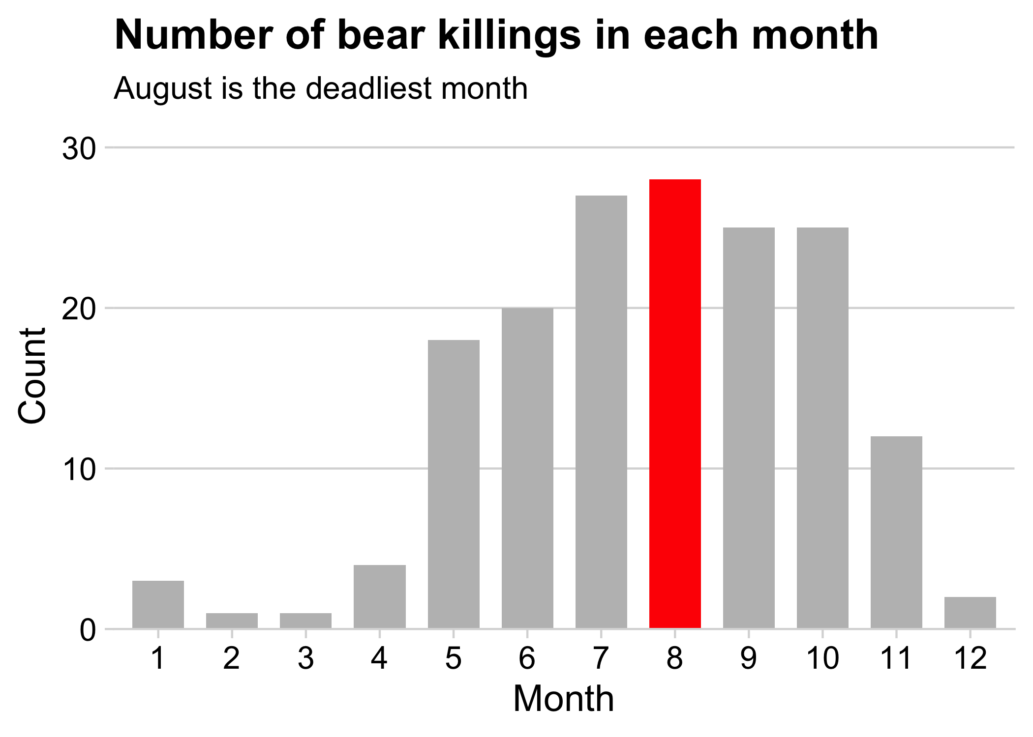
Your turn - practice plotting amounts

Create the following charts:

Data: bears

Data: milk_production

Break!

Stand up, Move around, Stretch!

Week 8: Factors, Amounts, & Proportions

1. Manipulating factors

2. Graphing amounts

3. Graphing proportions

Show proportions with:

Bar charts

Pie charts

Waffle charts

Stacked bars

# Format the data
milk_production %>%
  filter(year == 2017) %>%
  mutate(state = fct_other(state, keep = c('California', 'Wisconsin'))) %>%
  group_by(state) %>%
  summarise(milk_produced = sum(milk_produced)) %>%

  # Make the chart
  ggplot() +
  geom_col(
    aes(x = "", y = milk_produced, fill = state),
    width = 0.7,
    alpha = 0.8
  ) +
  scale_y_continuous(
    expand = expansion(mult = c(0, 0.05))
  ) +
  theme_minimal_hgrid() +
  labs(
    x = NULL,
    y = 'Milk produced (lbs)',
    fill = 'State',
    title = '2017 Milk Production\nby State'
  )

Stacked bars - Rotated also looks good

# Format the data
milk_production %>%
  filter(year == 2017) %>%
  mutate(state = fct_other(state, keep = c('California', 'Wisconsin'))) %>%
  group_by(state) %>%
  summarise(milk_produced = sum(milk_produced)) %>%

  # Make the chart
  ggplot() +
  geom_col(
    aes(x = milk_produced, y = "", fill = state),
    width = 0.7,
    alpha = 0.8
  ) +
  scale_x_continuous(
    expand = expansion(mult = c(0, 0.05))
  ) +
  theme_minimal_hgrid() +
  labs(
    y = NULL,
    x = 'Milk produced (lbs)',
    fill = 'State',
    title = '2017 Milk Production by State'
  )

Stacked bars - not great for more than a few categories

# Format the data
milk_production %>%
  filter(year == 2017) %>%
  mutate(
    state = fct_other(
      state,
      keep = c('California', 'Wisconsin', 'New York', 'Idaho')
    )
  ) %>%
  group_by(state) %>%
  summarise(milk_produced = sum(milk_produced))

# Make the chart
ggplot() +
  geom_col(
    aes(x = "", y = milk_produced, fill = state),
    width = 0.7,
    alpha = 0.8
  ) +
  scale_y_continuous(
    expand = expansion(mult = c(0, 0.05))
  ) +
  theme_minimal_vgrid() +
  labs(
    x = NULL,
    y = 'Milk produced (lbs)',
    fill = 'State',
    title = '2017 Milk Production\nby State'
  )

Dodged bars

Better for part-to-whole comparison

# Format the data
milk_production %>%
  filter(year == 2017) %>%
  mutate(state = fct_other(state, keep = c('California', 'Wisconsin'))) %>%
  group_by(state) %>%
  summarise(milk_produced = sum(milk_produced)) %>%
  mutate(state = fct_reorder(state, milk_produced)) %>%

  # Make the chart
  ggplot() +
  geom_col(
    aes(x = milk_produced, y = state),
    width = 0.7,
    alpha = 0.8
  ) +
  scale_x_continuous(
    expand = expansion(mult = c(0, 0.05))
  ) +
  theme_minimal_vgrid() +
  labs(
    x = 'Milk produced (lbs)',
    y = 'State',
    title = '2017 Milk Production by State'
  )

Okay:

Better:

Dodged bars

milk_production %>%
  filter(year %in% c(1970, 2017)) %>%
  mutate(state = fct_other(state, keep = c('California', 'Wisconsin'))) %>%
  group_by(year, state) %>%
  summarise(milk_produced = sum(milk_produced)) %>%

  # Make the chart
  ggplot() +
  geom_col(
    aes(x = milk_produced, y = as.factor(year), fill = state),
    position = 'dodge',
    width = 0.7,
    alpha = 0.8
  ) +
  scale_x_continuous(
    expand = expansion(mult = c(0, 0.05))
  ) +
  theme_minimal_vgrid() +
  labs(
    x = 'Milk produced (lbs)',
    y = 'Year',
    fill = 'State',
    title = '1970 & 2017 Milk Production by State'
  )

Better for comparing total:

Better for comparing parts:

Where stacking is useful

https://fivethirtyeight.com/features/the-dollar-and-cents-case-against-hollywoods-exclusion-of-women/

- 2 to 3 groups

- Proportions over time

Where stacking is useful

https://www.perceptualedge.com/blog/?p=2239

- 2 to 3 groups

- Proportions over time

The Notorious P-I-E

Start with a bar chart

# Format the data
milk_production %>%
  filter(year == 2017) %>%
  mutate(state = fct_other(state, keep = c('California', 'Wisconsin'))) %>%
  group_by(state) %>%
  summarise(milk_produced = sum(milk_produced)) %>%

  # Make the chart
  ggplot() +
  geom_col(
    aes(x = "", y = milk_produced, fill = state),
    width = 0.7,
    alpha = 0.8
  ) +
  theme_minimal_hgrid() +
  labs(
    x = NULL,
    y = 'Milk produced (lbs)',
    fill = 'State',
    title = '2017 Milk Production\nby State'
  )

The Notorious P-I-E

Convert bar to pie with coord_polar()

# Format the data
milk_production %>%
  filter(year == 2017) %>%
  mutate(state = fct_other(state, keep = c('California', 'Wisconsin'))) %>%
  group_by(state) %>%
  summarise(milk_produced = sum(milk_produced)) %>%

  # Make the chart
  ggplot() +
  geom_col(
    aes(x = "", y = milk_produced, fill = state),
    width = 0.7,
    alpha = 0.8
  ) +
  coord_polar(theta = "y") +
  theme_minimal_hgrid() +
  labs(
    x = NULL,
    y = 'Milk produced (lbs)',
    fill = 'State',
    title = '2017 Milk Production by State'
  )

# Format the data
milk_production %>%
  filter(year == 2017) %>%
  mutate(state = fct_other(state, keep = c('California', 'Wisconsin'))) %>%
  group_by(state) %>%
  summarise(milk_produced = sum(milk_produced)) %>%
  arrange(desc(state)) %>%
  mutate(
    p = 100 * (milk_produced / sum(milk_produced)),
    label = str_c(round(p), '%')
  ) %>%

  # Make the chart
  ggplot() +
  geom_col(
    aes(x = "", y = milk_produced, fill = state),
    width = 0.7,
    alpha = 0.8
  ) +
  geom_text(
    aes(x = "", y = milk_produced, label = label),
    color = "white",
    size = 6,
    position = position_stack(vjust = 0.5)
  ) +
  coord_polar(theta = "y") +
  theme_map() +
  labs(
    x = NULL,
    y = NULL,
    fill = 'State',
    title = '2017 Milk Production by State'
  )

The Notorious P-I-E

Final chart with labels & theme_map()

Pies are still useful if the sum of components matters

The best pies are square pies

https://eagereyes.org/blog/2016/a-reanalysis-of-a-study-about-square-pie-charts-from-2009

Waffle plots

library(waffle)

# Format the data
milk_production %>%
  filter(year == 2017) %>%
  mutate(state = fct_other(state, keep = c('California', 'Wisconsin'))) %>%
  group_by(state) %>%
  summarise(milk_produced = sum(milk_produced)) %>%
  mutate(milk_produced = milk_produced / 10^9) %>%

  # Make the chart
  ggplot() +
  geom_waffle(
    aes(fill = state, values = milk_produced),
    color = "white",
    size = 1,
    n_rows = 10
  ) +
  scale_x_discrete(expand = c(0, 0)) +
  scale_y_discrete(expand = c(0, 0)) +
  theme_minimal() +
  labs(
    fill = 'State',
    x = NULL,
    y = NULL,
    title = '2017 Milk Production by State',
    subtitle = '(1 square = 1 billion lbs)'
  )

Use values between 100 - 1,000

(You don’t want 1,000,000,000 boxes!)

#> # A tibble: 3 × 2
#>   state      milk_produced
#>   <fct>              <dbl>
#> 1 California          39.8
#> 2 Wisconsin           30.3
#> 3 Other              145.

Waffle plots

library(waffle)

# Format the data
milk_production %>%
  filter(year == 2017) %>%
  mutate(state = fct_other(state, keep = c('California', 'Wisconsin'))) %>%
  group_by(state) %>%
  summarise(milk_produced = sum(milk_produced)) %>%
  mutate(milk_produced = milk_produced / 10^9) %>%

  # Make the chart
  ggplot() +
  geom_waffle(
    aes(fill = state, values = milk_produced),
    color = "white",
    size = 1,
    n_cols = 10,
    flip = TRUE
  ) +
  scale_x_discrete(expand = c(0, 0)) +
  scale_y_discrete(expand = c(0, 0)) +
  theme_minimal() +
  labs(
    fill = 'State',
    x = NULL,
    y = NULL,
    title = '2017 Milk Production by State',
    subtitle = '(1 square = 1 billion lbs)'
  )

Use flip = TRUE for vertical

#> # A tibble: 3 × 2
#>   state      milk_produced
#>   <fct>              <dbl>
#> 1 California          39.8
#> 2 Wisconsin           30.3
#> 3 Other              145.

library(waffle)

# Format the data
milk_production %>%
  filter(year %in% c(1970, 2017)) %>%
  mutate(state = fct_other(state, keep = c('California', 'Wisconsin'))) %>%
  group_by(year, state) %>%
  summarise(milk_produced = sum(milk_produced)) %>%
  mutate(milk_produced = milk_produced / 10^9) %>%

  # Make the chart
  ggplot() +
  geom_waffle(
    aes(fill = state, values = milk_produced),
    color = "white",
    size = 1,
    n_rows = 10,
    flip = TRUE
  ) +
  facet_wrap(vars(year), strip.position = 'bottom') +
  scale_x_discrete(expand = c(0, 0)) +
  scale_y_discrete(expand = c(0, 0)) +
  theme_minimal() +
  labs(
    fill = 'State',
    x = NULL,
    y = NULL,
    title = '1970 & 2017 Milk Production by State',
    subtitle = '(1 square = 1 billion lbs)'
  )

Use facet_wrap for side-by-side waffles

#> # A tibble: 3 × 2
#>   state      milk_produced
#>   <fct>              <dbl>
#> 1 California          39.8
#> 2 Wisconsin           30.3
#> 3 Other              145.

Stacked bars

Dodged bars

Pie chart

Waffle chart

Your turn

Using the wildlife_impacts data, create plots that shows the proportion of incidents that occur at each different time of day.

For this exercise, you can remove NA values.

Try to create the following plots:

Stacked bars
Dodged bars
Pie chart
Waffle chart

To get started, you’ll need to first summarize the data:

wildlife_summary <- wildlife_impacts %>%
  filter(!is.na(time_of_day)) %>%
  count(time_of_day)

wildlife_summary

#> # A tibble: 4 × 2
#>   time_of_day     n
#>   <chr>       <int>
#> 1 Dawn         1270
#> 2 Day         25123
#> 3 Dusk         1717
#> 4 Night       12735

Quiz 3

Next projects due:

- Mini project 2: Exploring Data (Due 10/25)

- Initial Report (Due 11/01)

Today’s data

New packages

Week 8: Factors, Amounts, & Proportions

1. Manipulating factors

2. Graphing amounts

3. Graphing proportions

Week 8: Factors, Amounts, & Proportions

1. Manipulating factors

2. Graphing amounts

3. Graphing proportions

Sorting in ggplot is done by reordering factors

Two ways to sort

Two ways to sort

Common situations for modifying / reording factors:

1. Reorder factors based on another numerical variable

2. Reorder factors manually

3. Modify factors manually

4. What if there are too many factor levels?

1. Reorder factors based on another numerical variable

2. Reorder factors manually

2. Reorder factors manually with fct_relevel()

3. Modify factors manually

3. Modify factors manually with fct_recode()

2 & 3. Modify and reorder factors manually

4. What if there are too many factor levels?

4. What if there are too many factor levels?

4. What if there are really too many factor levels?

4. What if there are really too many factor levels?

4. What if there are really too many factor levels?

Your turn - practice manipulating factors

Week 8: Factors, Amounts, & Proportions

1. Manipulating factors

2. Graphing amounts

3. Graphing proportions

Show amounts with:

Bars are good for highlighting specific categories

Use lollipops when:

- The bars are overwhelming - You’re not highlighting categories

Or use dots and don’t set axis to 0

How to make a Bar chart

Filling the bars with color

Filling the bars with color

How to make a Dot chart

How to make a Lollipop chart

Your turn - practice plotting amounts

Week 8: Factors, Amounts, & Proportions

1. Manipulating factors

2. Graphing amounts

3. Graphing proportions

Show proportions with:

Stacked bars

Stacked bars - Rotated also looks good

Stacked bars - not great for more than a few categories

Where stacking is useful

Where stacking is useful

The Notorious P-I-E

The Notorious P-I-E

Pies are still useful if the sum of components matters

The best pies are square pies

Your turn

2. Reorder factors manually with `fct_relevel()`

3. Modify factors manually with `fct_recode()`

- The bars are overwhelming
- You’re not highlighting categories