college_all_ages <- read_csv(file.path('data', 'college_all_ages.csv'))
gapminder <- read_csv(file.path('data', 'gapminder.csv'))
marathon <- read_csv(file.path('data', 'marathon.csv'))
milk_production <- read_csv(file.path('data', 'milk_production.csv'))
internet_regions <- read_csv(file.path('data', 'internet_users_region.csv'))
Comparisons
EMSE 4572/6572: Exploratory Data Analysis
John Paul Helveston
October 21, 2026
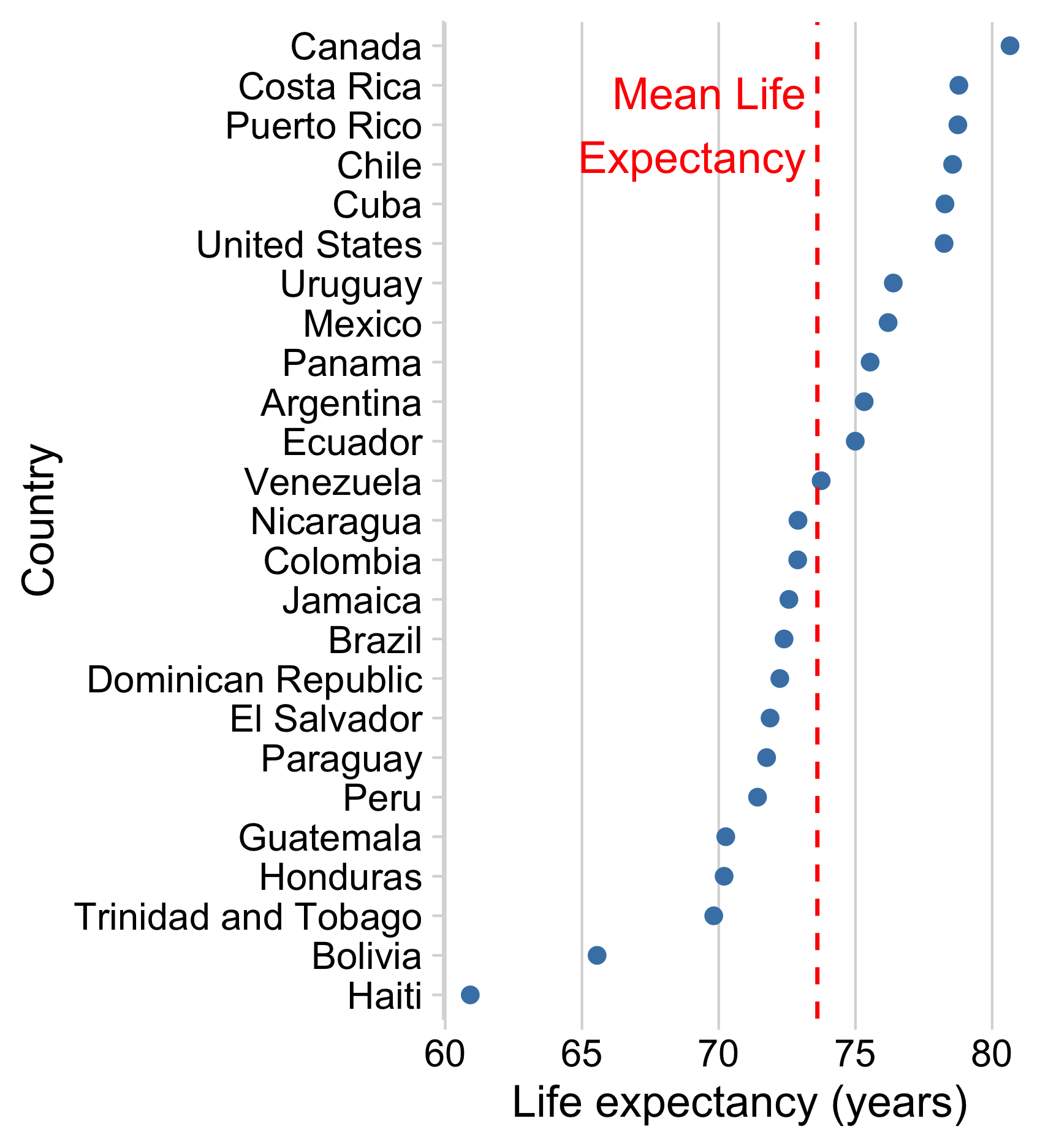
Use reference lines to add context to chart
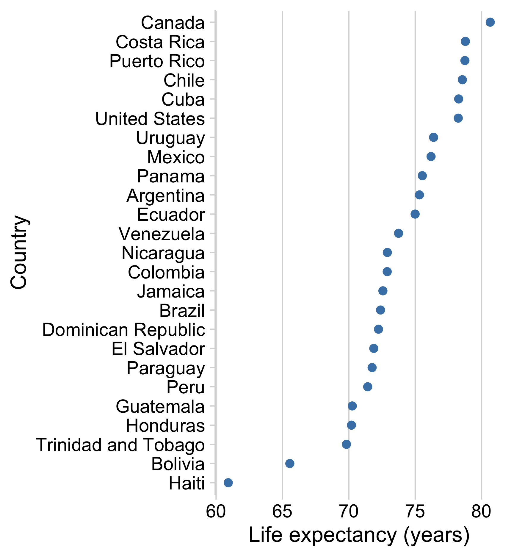
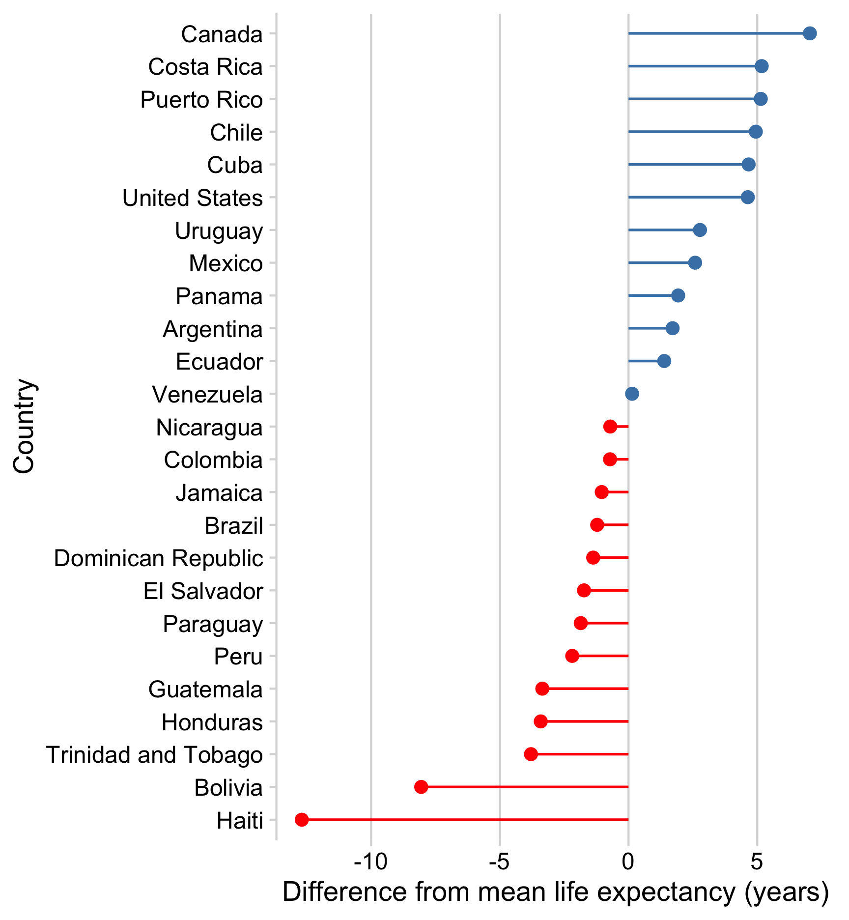
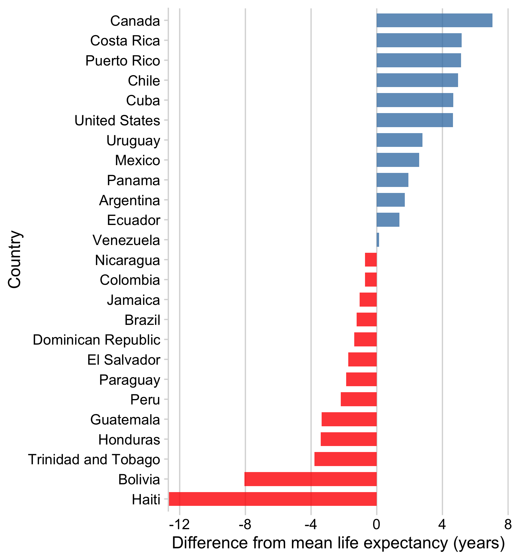
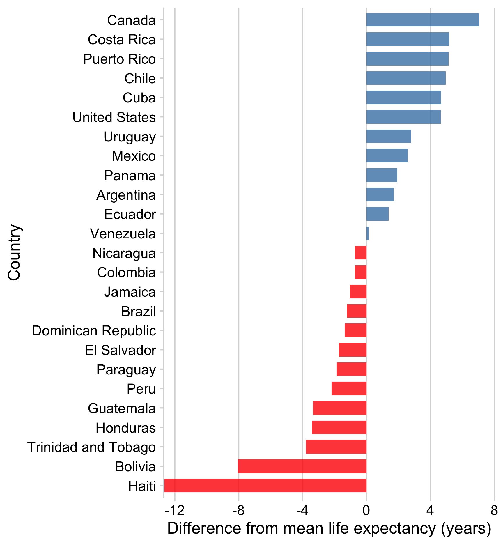
Or make zero the reference line
How to add a reference line
Add horizontal line with geom_hline()
Add vertical line with geom_vline()
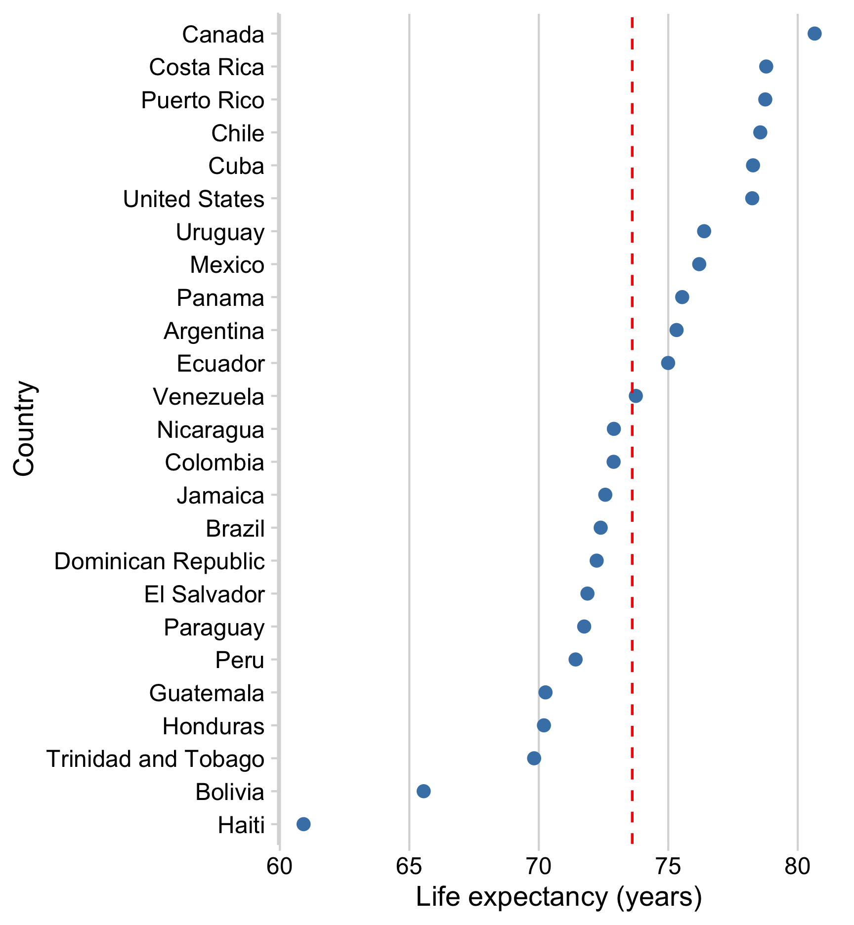
How to add a reference line
Add text with annotate()
ggplot(gapminder_americas) +
  geom_point(
    aes(x = lifeExp, y = country),
    color = 'steelblue',
    size = 2.5
  ) +
  geom_vline(
    xintercept = mean(gapminder_americas$lifeExp),
    color = 'red',
    linetype = 'dashed'
  ) +
  annotate(
    'text',
    x = 73.2,
    y = 'Puerto Rico',
    color = 'red',
    hjust = 1,
    label = 'Mean Life\nExpectancy'
  ) +
  theme_minimal_vgrid() +
  labs(x = 'Life expectancy (years)', y = 'Country')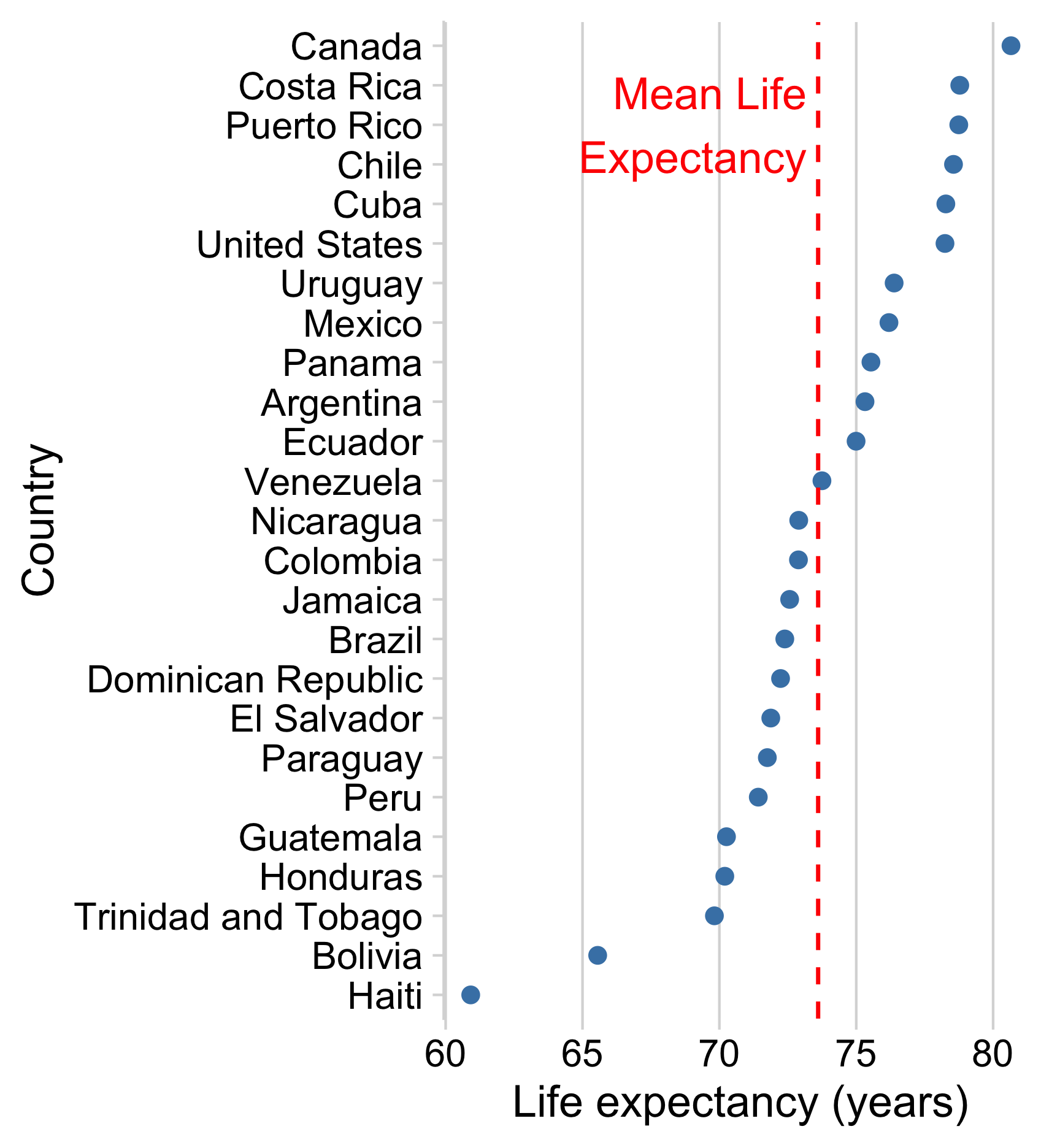
How to make zero the reference point
15:00
Your turn - comparing to a reference
Make a ranking chart and either a) add a reference line or b) show the ranking as the difference from a reference (e.g. the mean). Use any dataset you want in the “data” folder (examples below using milk_production.csv)
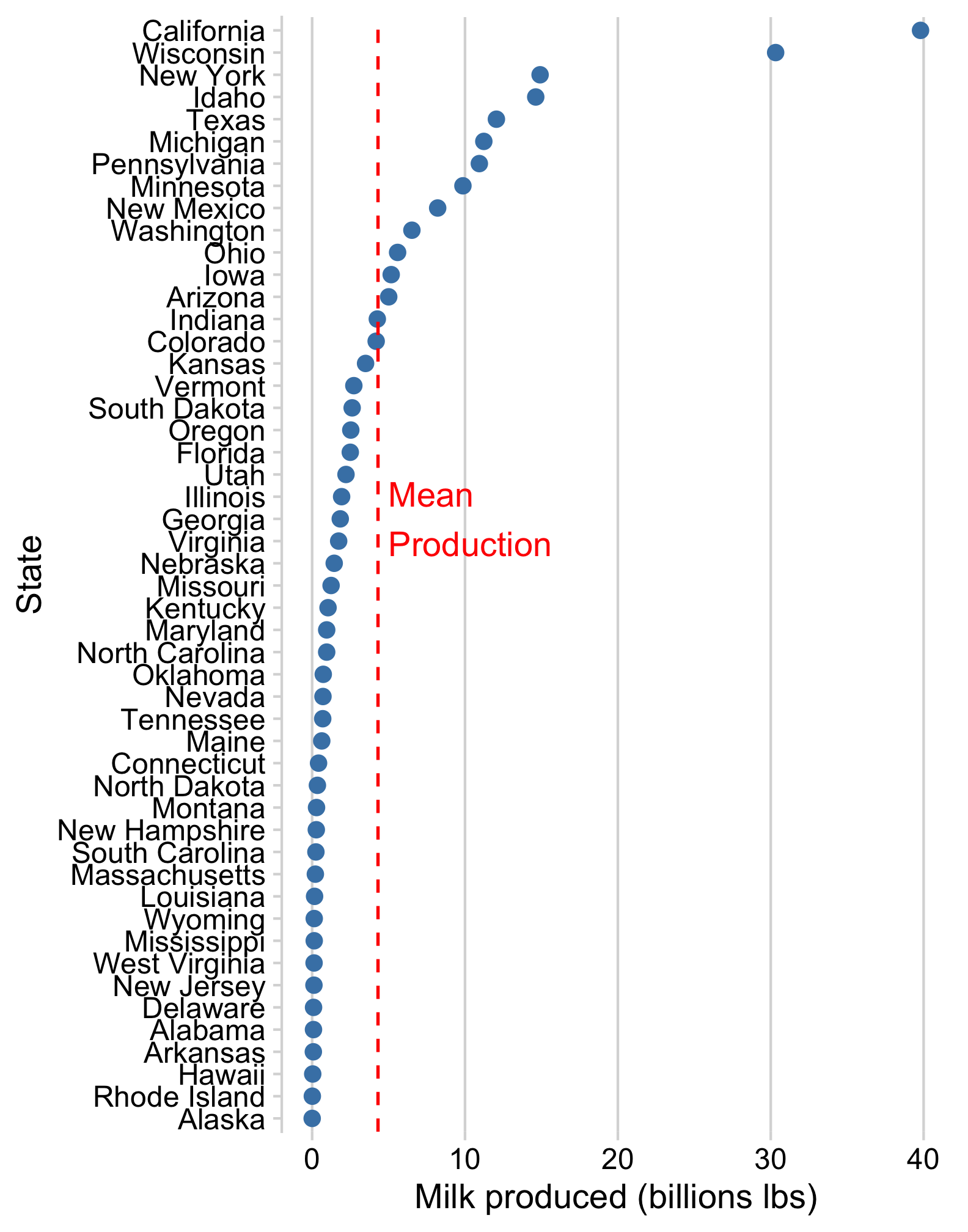
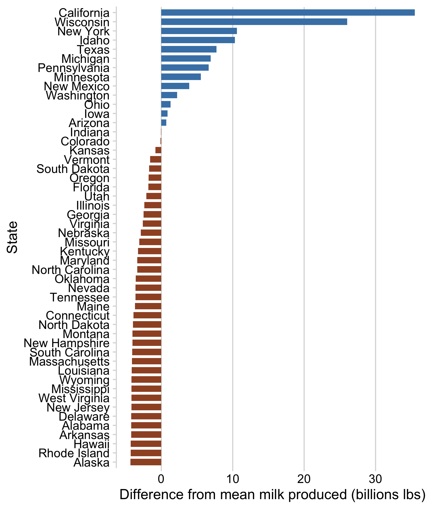
Neither of these charts are great
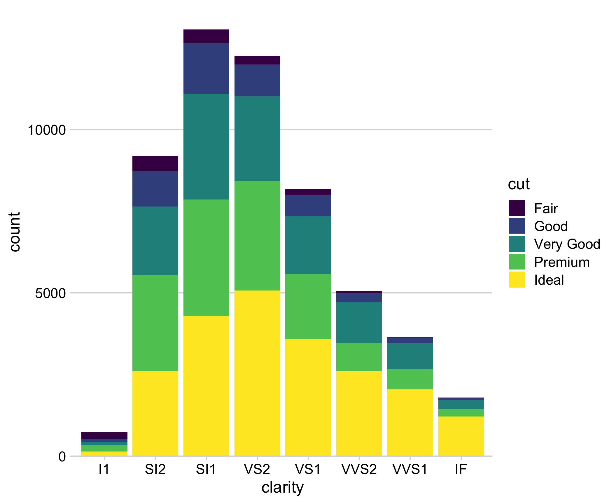
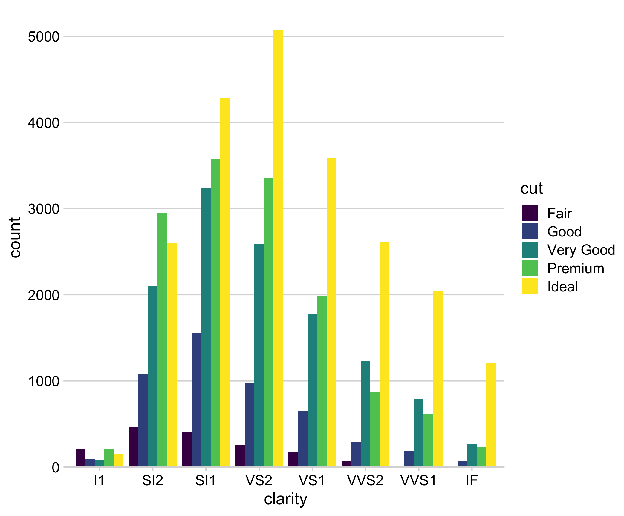
“Parallel Coordinates” plots work well
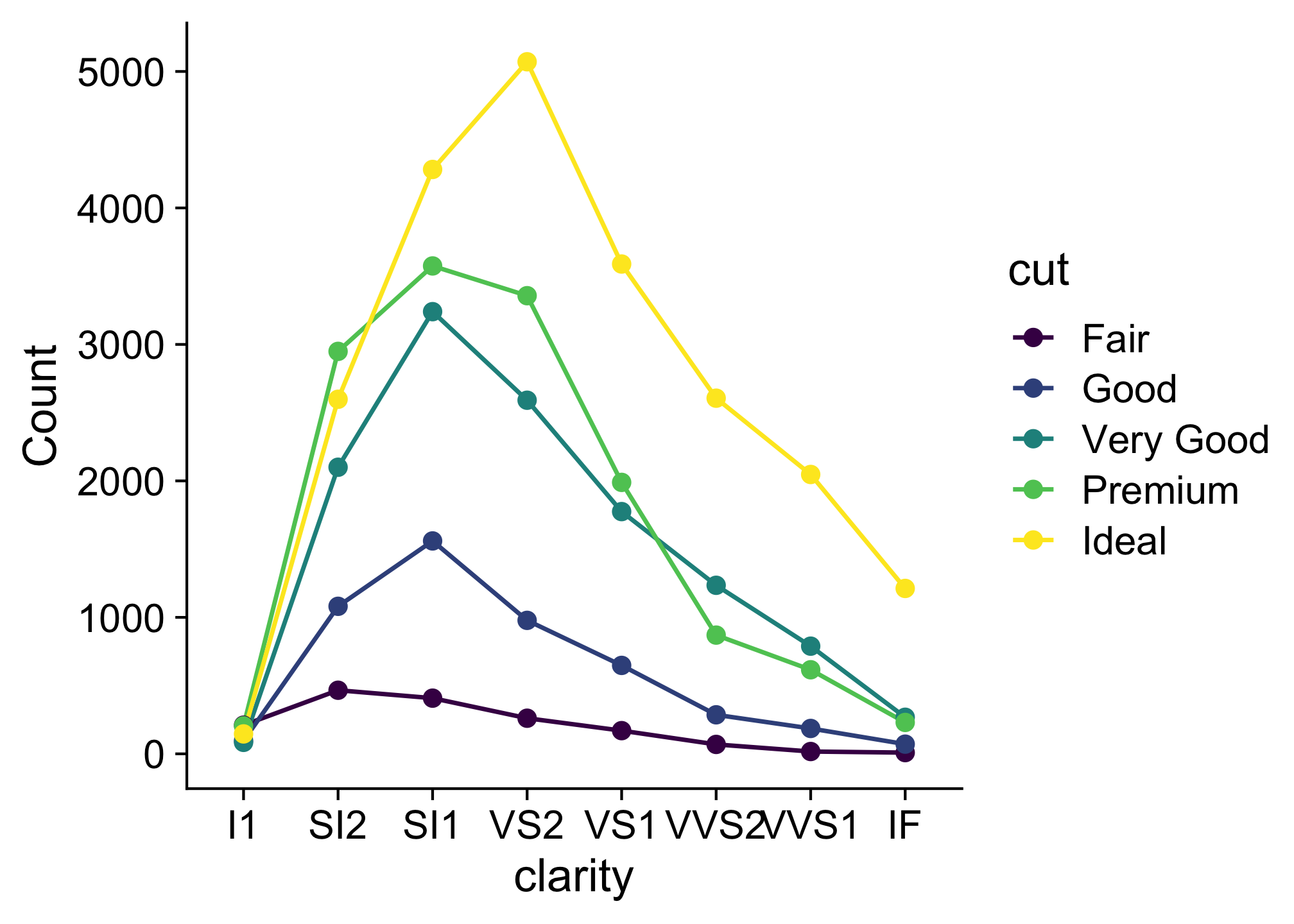
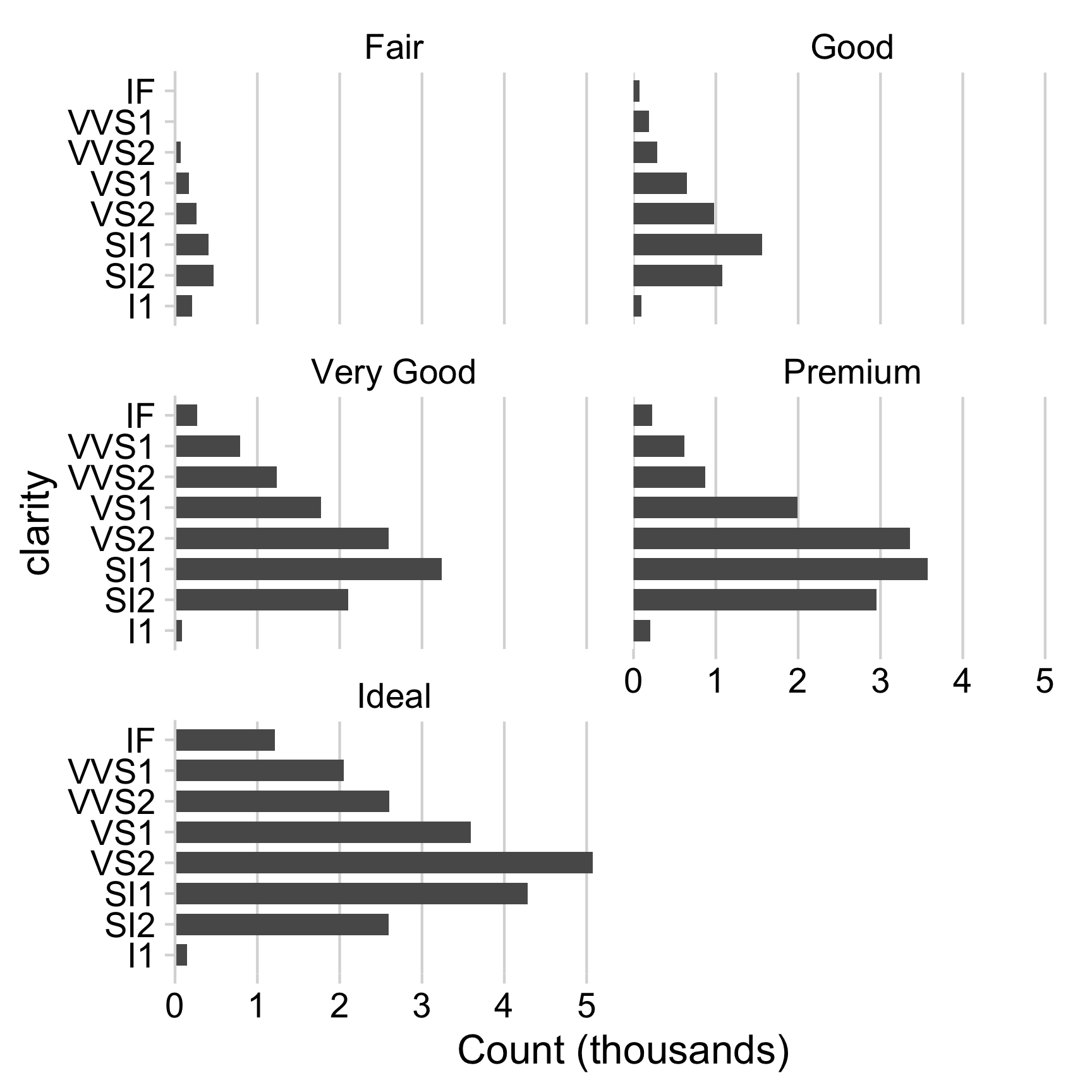
Consider facets for comparing across categories

Consider facets for comparing across categories
diamonds %>%
  count(clarity, cut) %>%
  mutate(n = n / 1000) %>%
  ggplot() +
  geom_col(aes(x = clarity, y = n), width = 0.7) +
  facet_wrap(vars(cut), ncol = 2) +
  coord_flip() +
  scale_y_continuous(
    expand = expansion(mult = c(0, 0.05))
  ) +
  theme_minimal_vgrid(font_size = 16) +
  labs(y = "Count (thousands)")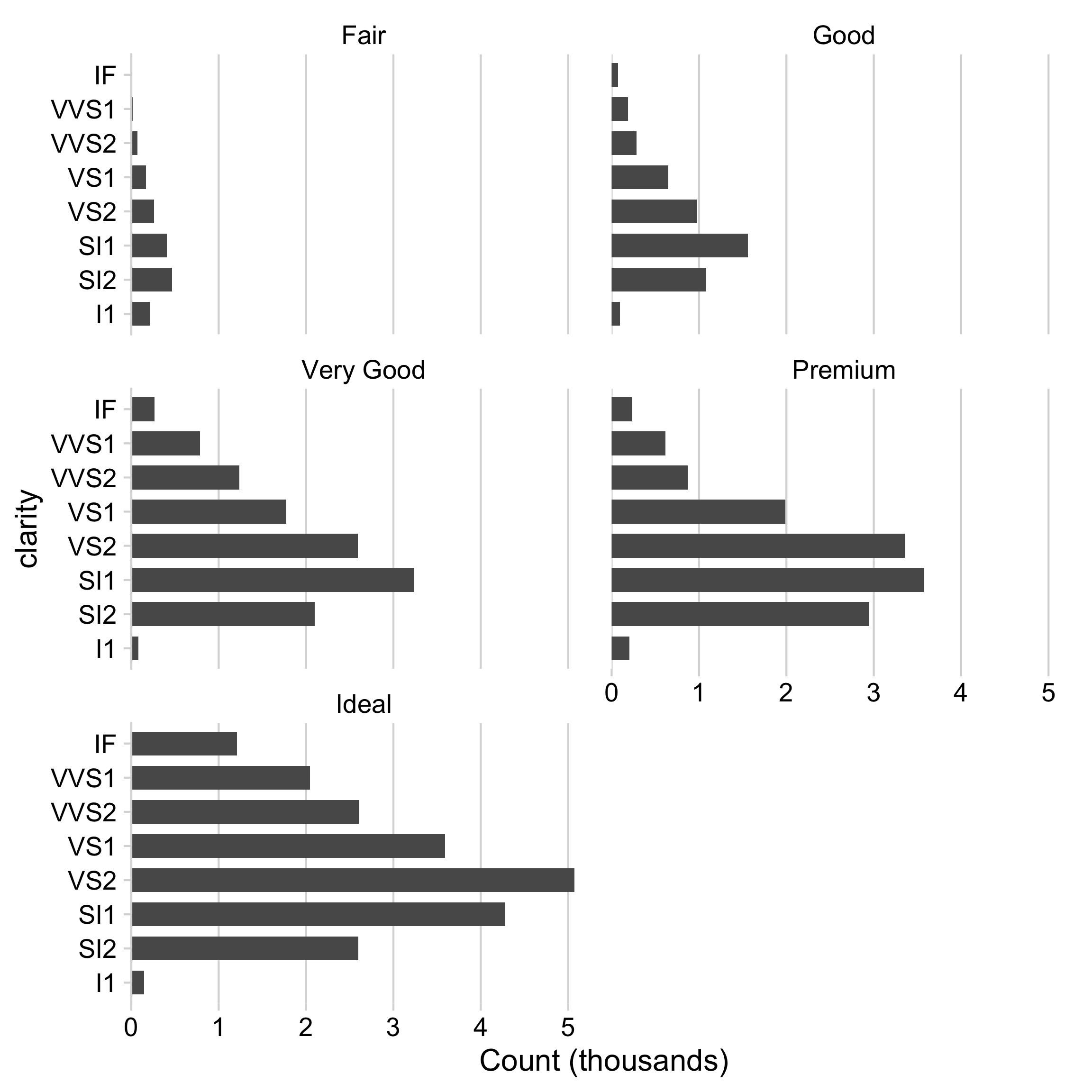
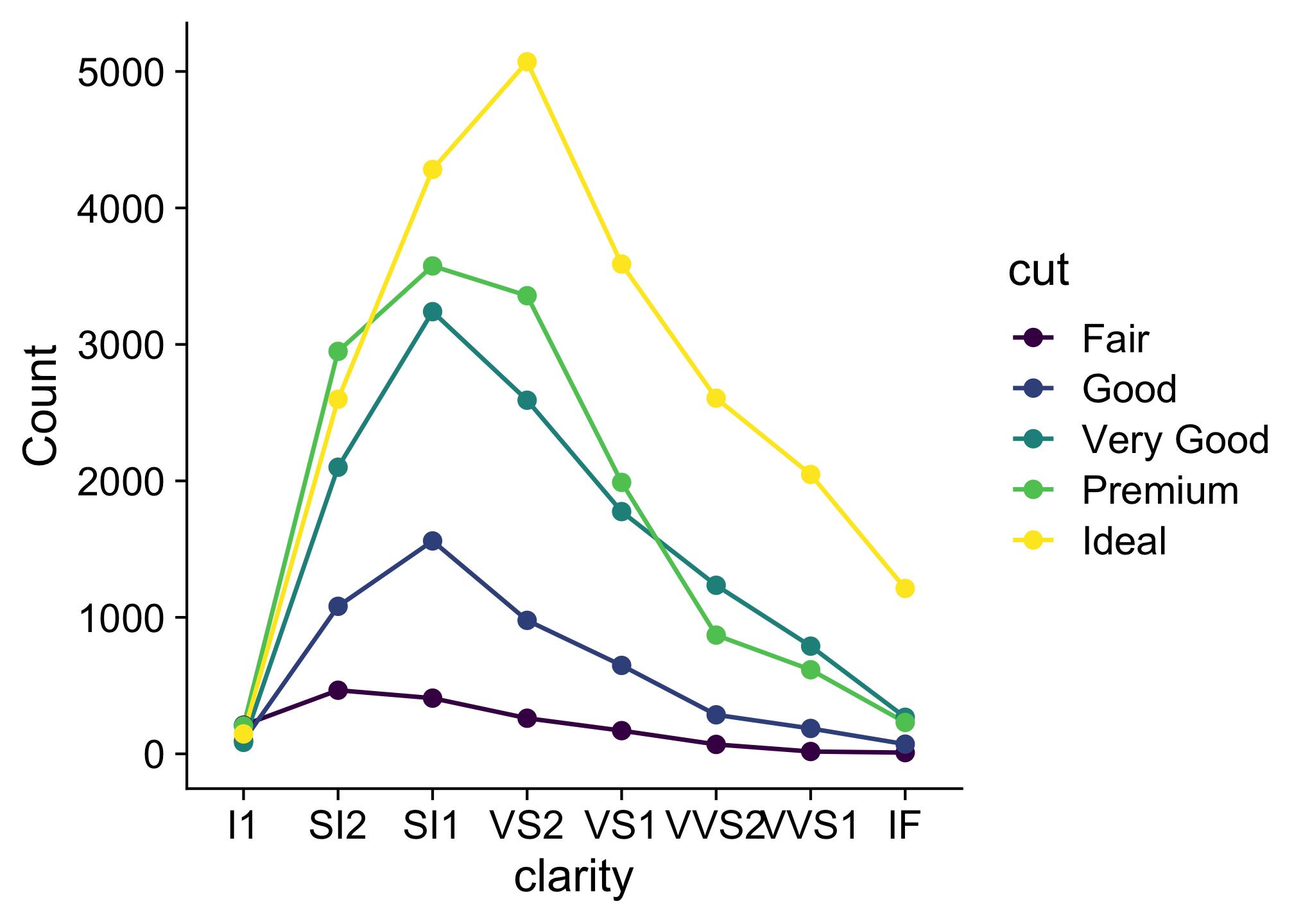
When comparing across multiple categories, consider:
Parallel coordinates charts
Faceting
When comparing only 2 things,
dodged bars are a good starting point
#> # A tibble: 6 × 3
#> # Groups:   year [2]
#>    year state      milk_produced
#>   <dbl> <fct>              <dbl>
#> 1  1970 California          9.46
#> 2  1970 Wisconsin          18.4
#> 3  1970 Other              89.1
#> 4  2017 California         39.8
#> 5  2017 Wisconsin          30.3
#> 6  2017 Other             145.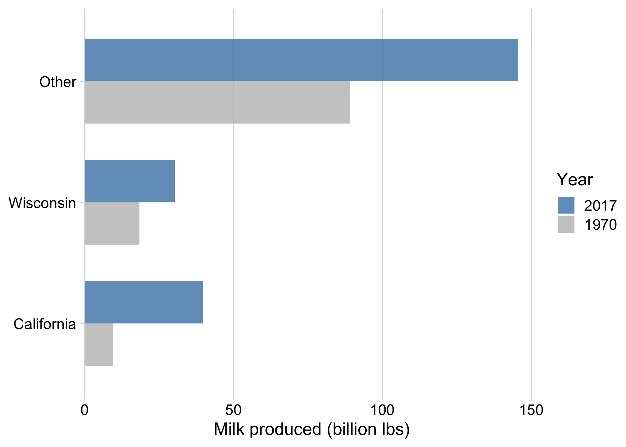
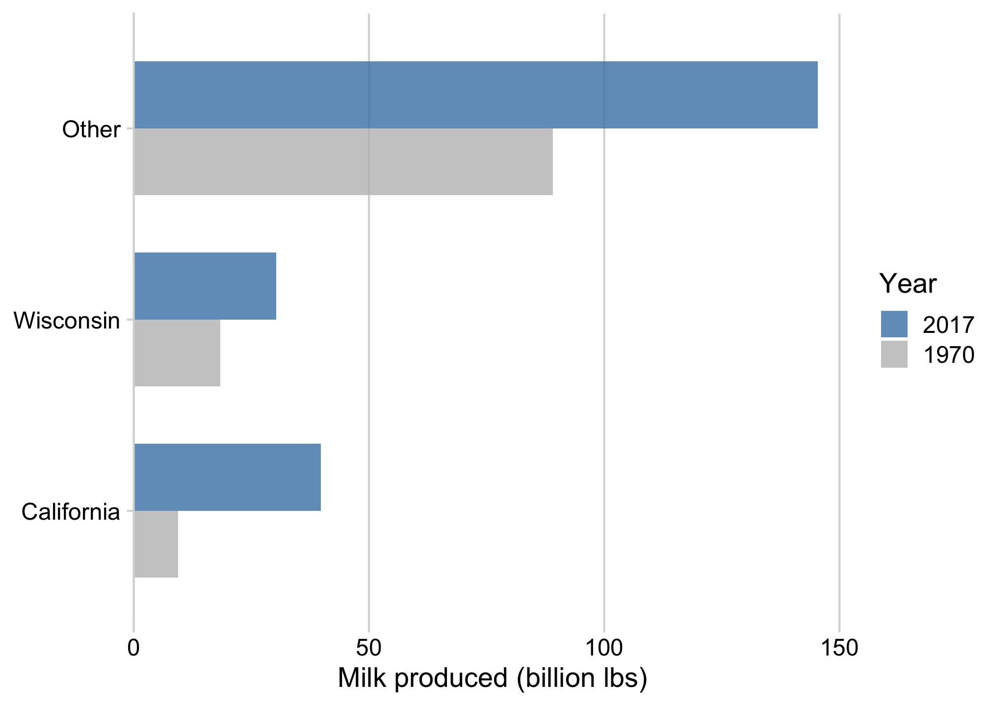
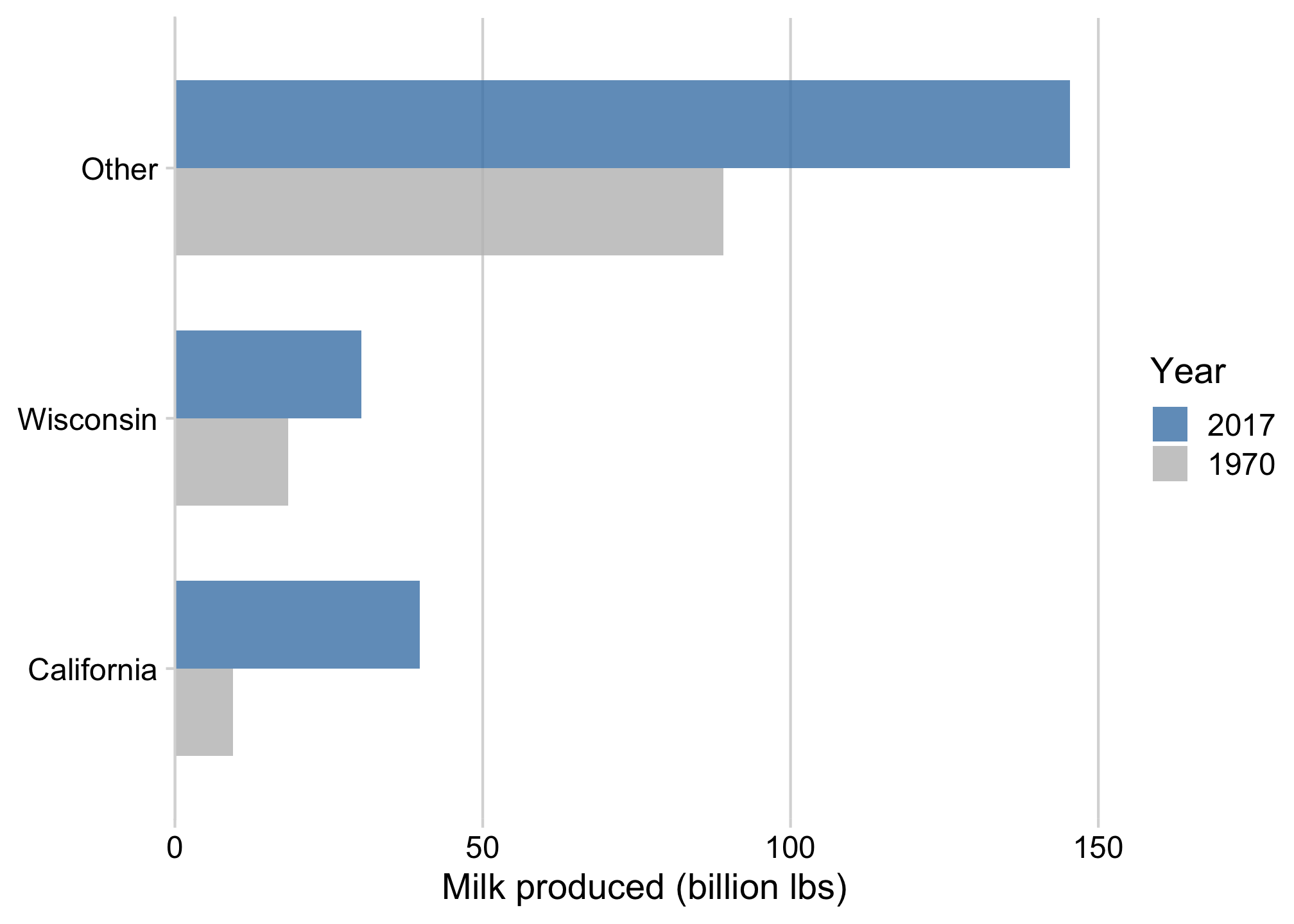
When comparing only 2 things,
dodged bars are a good starting point
ggplot(milk_compare) +
  geom_col(
    aes(
      x = milk_produced,
      y = state,
      fill = as.factor(year)
    ),
    width = 0.7,
    alpha = 0.8,
    position = 'dodge'
  ) +
  scale_fill_manual(
    values = c('grey', 'steelblue'),
    guide = guide_legend(reverse = TRUE)
  ) +
  scale_x_continuous(
    expand = expansion(mult = c(0, 0.05))
  ) +
  theme_minimal_vgrid() +
  labs(
    x = 'Milk produced (billion lbs)',
    y = NULL,
    fill = 'Year'
  )
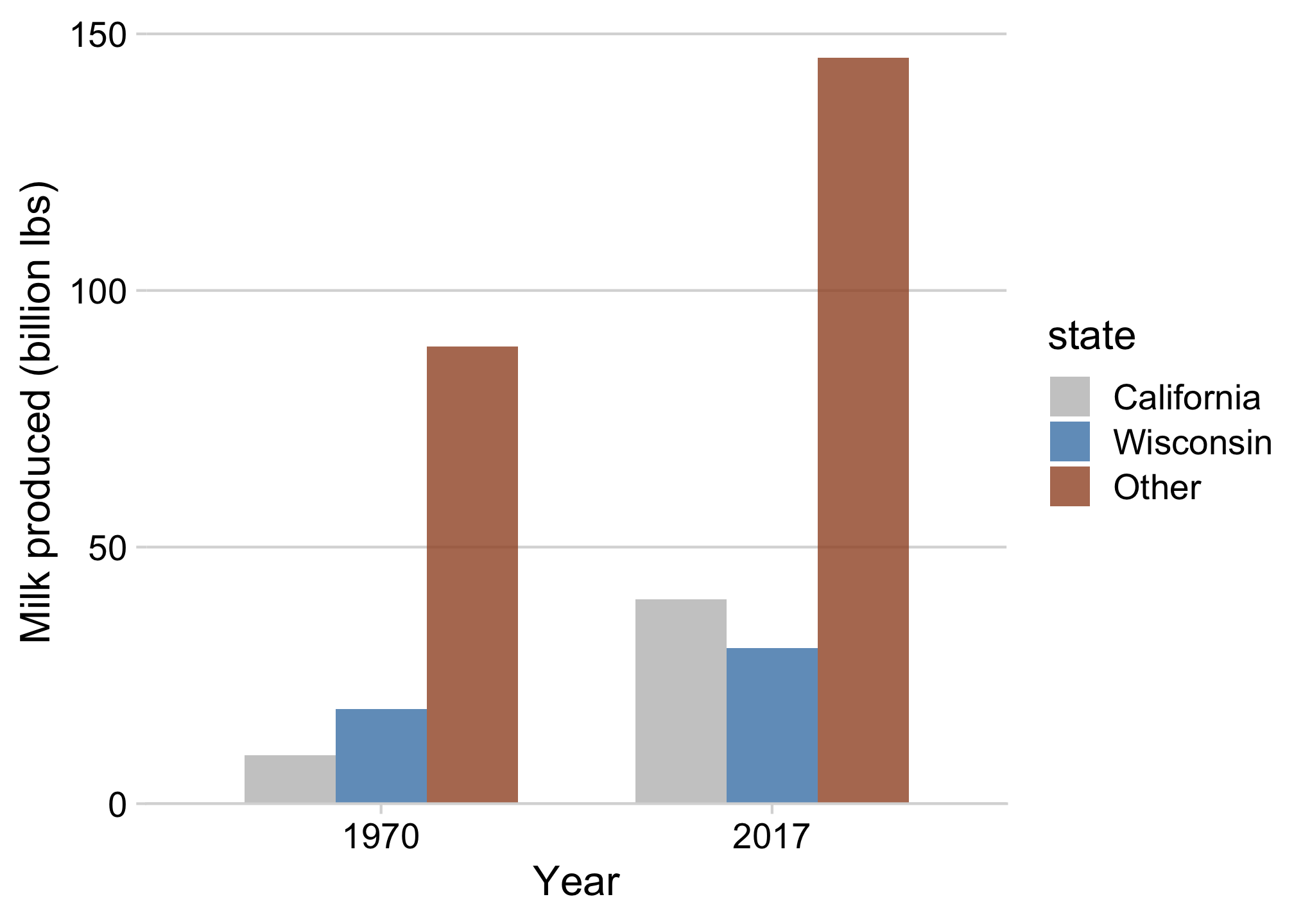
Avoid putting >2 categories in legend (if possible)

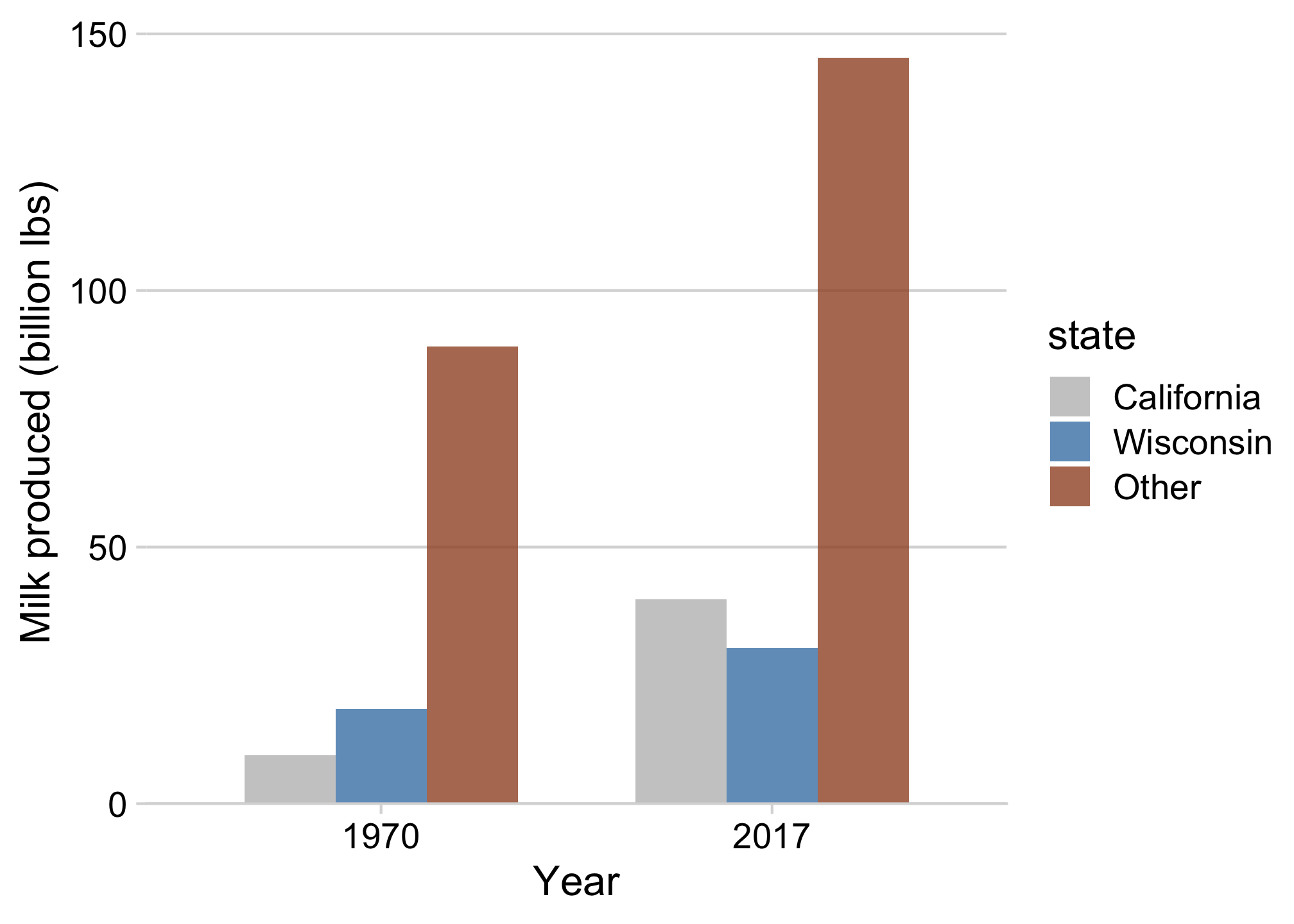

Or use facets to get rid of the legend!
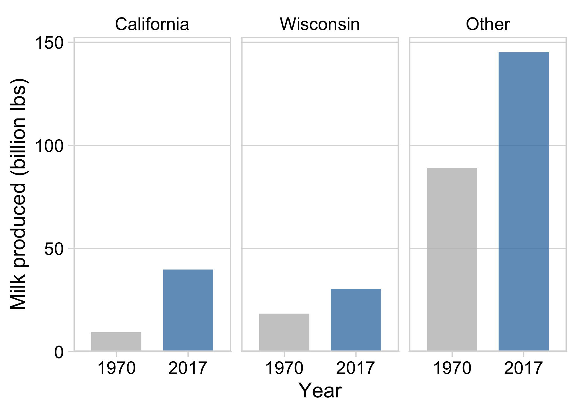
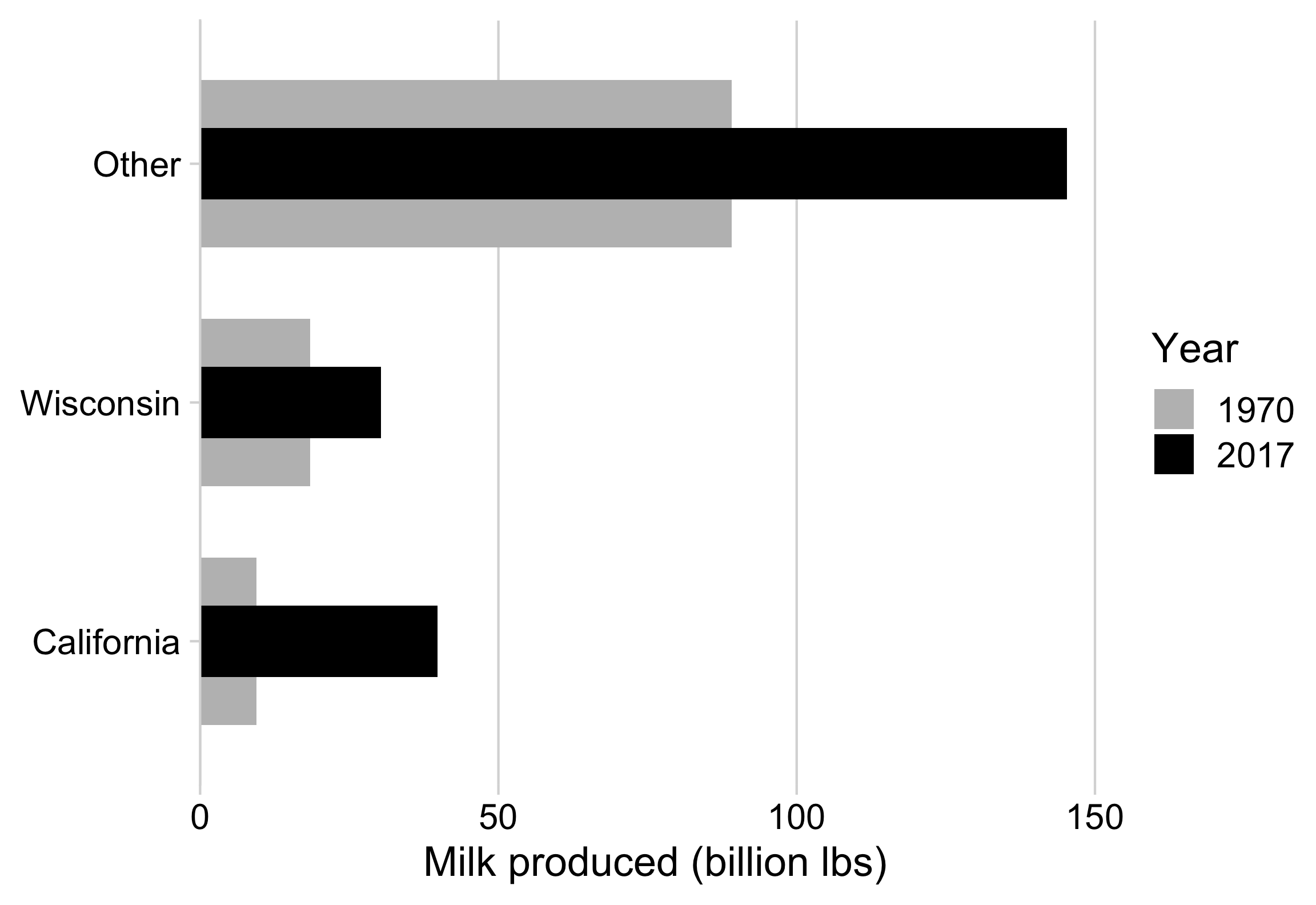
“Bullet” charts are also effective for comparing 2 things
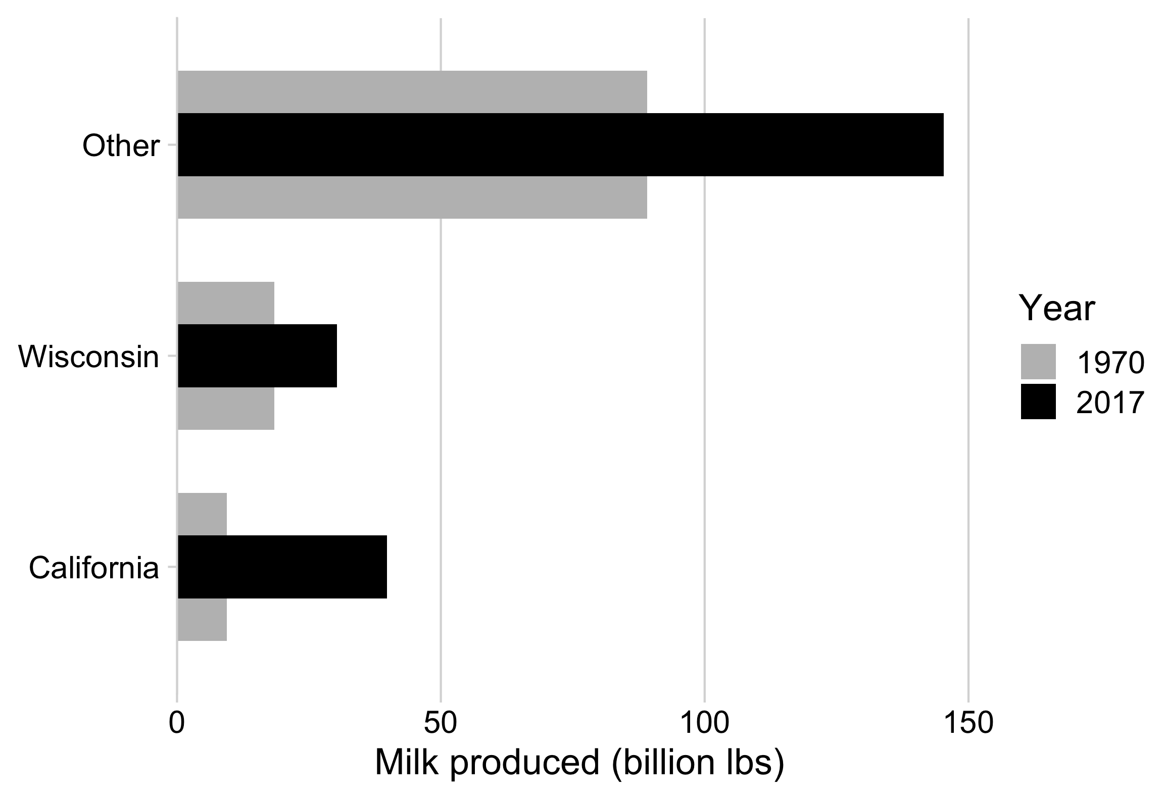
How to make a “bullet” chart
milk_compare %>%
  pivot_wider(
    names_from = year,
    values_from = milk_produced
  ) %>%
  ggplot() +
  geom_col(
    aes(x = `1970`, y = state, fill = '1970'),
    width = 0.7
  ) +
  geom_col(
    aes(x = `2017`, y = state, fill = '2017'),
    width = 0.3
  ) +
  scale_fill_manual(
    values = c('grey', 'black')
  ) +
  scale_x_continuous(
    expand = expansion(mult = c(0, 0.05))
  ) +
  theme_minimal_vgrid(font_size = 18) +
  labs(
    x = 'Milk produced (billion lbs)',
    y = NULL,
    fill = "Year"
  )
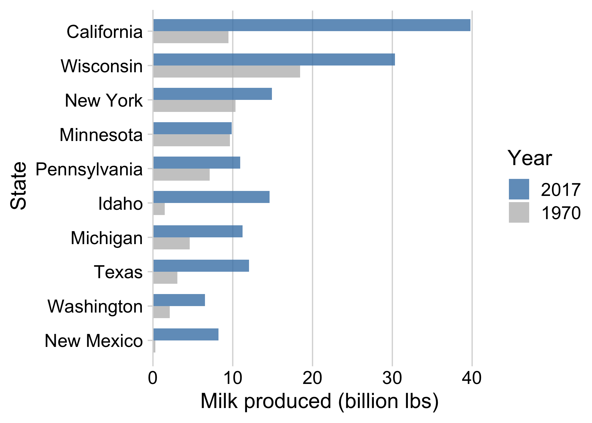
With more than 2 things, dodged bars can get confusing
Still comparing 2 time periods, but across 10 categories
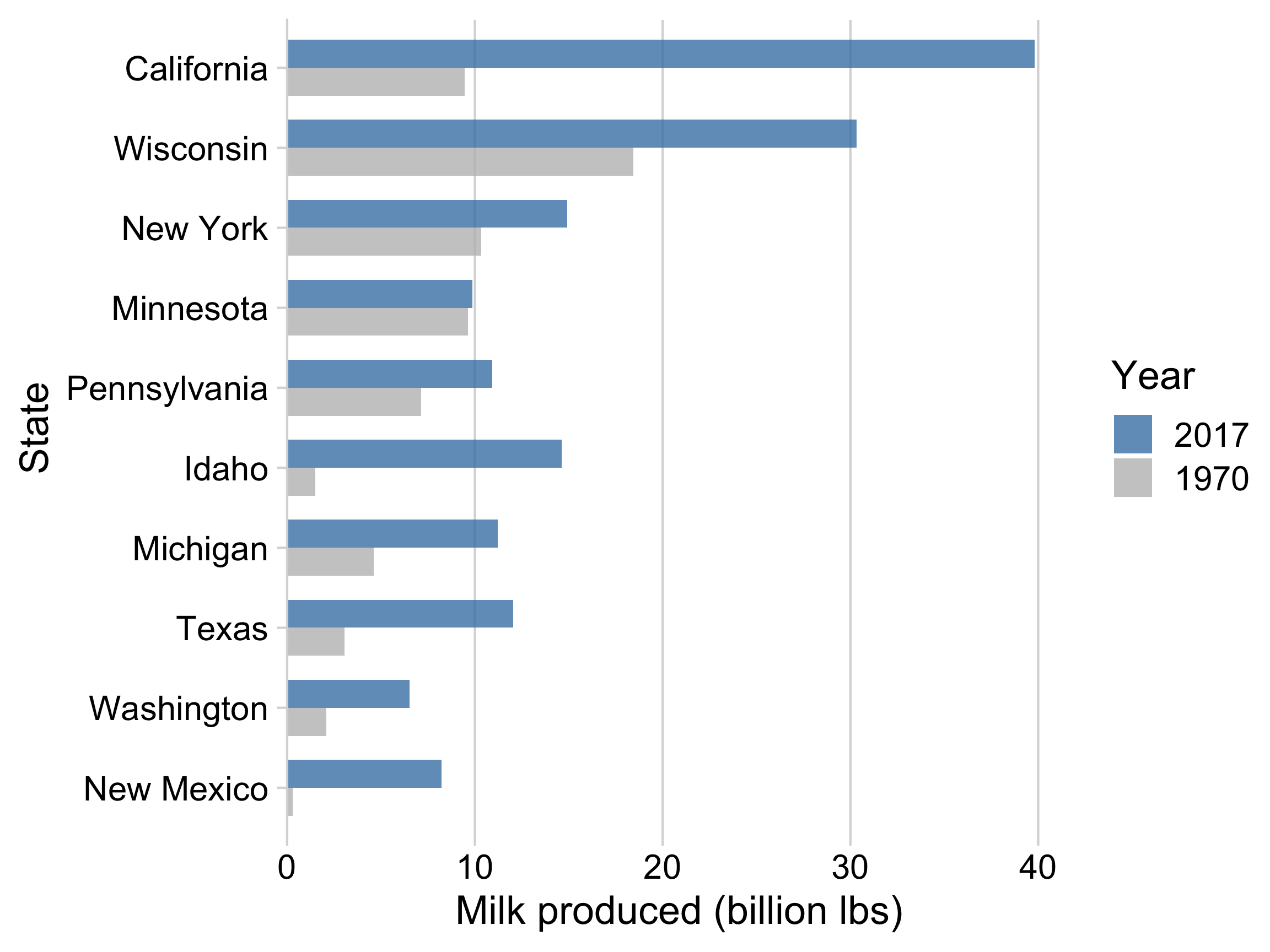
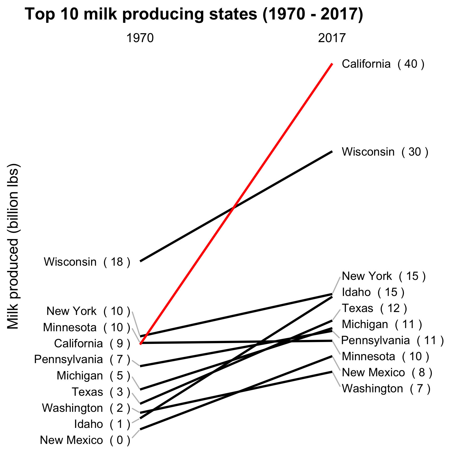
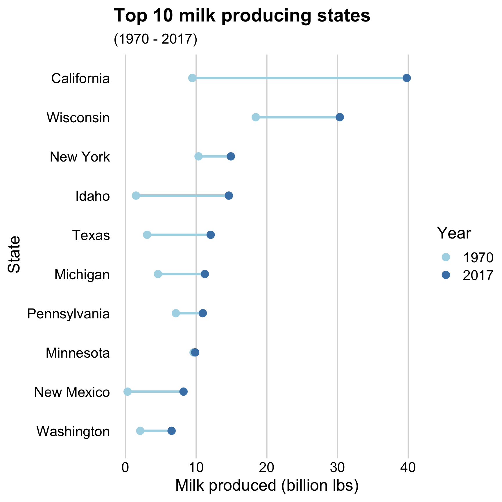
Strategies for comparing 2 things across more than 2 categories
Dodged bars 😢
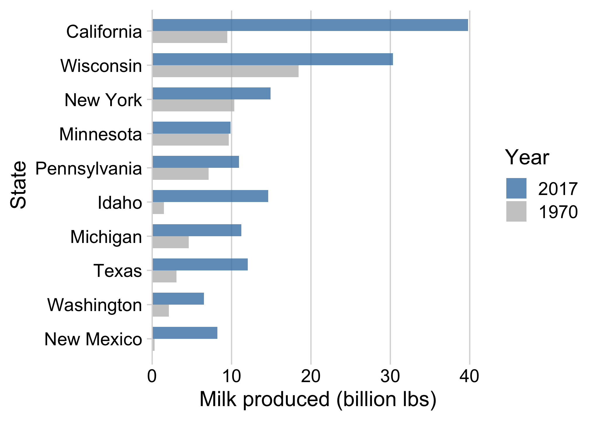
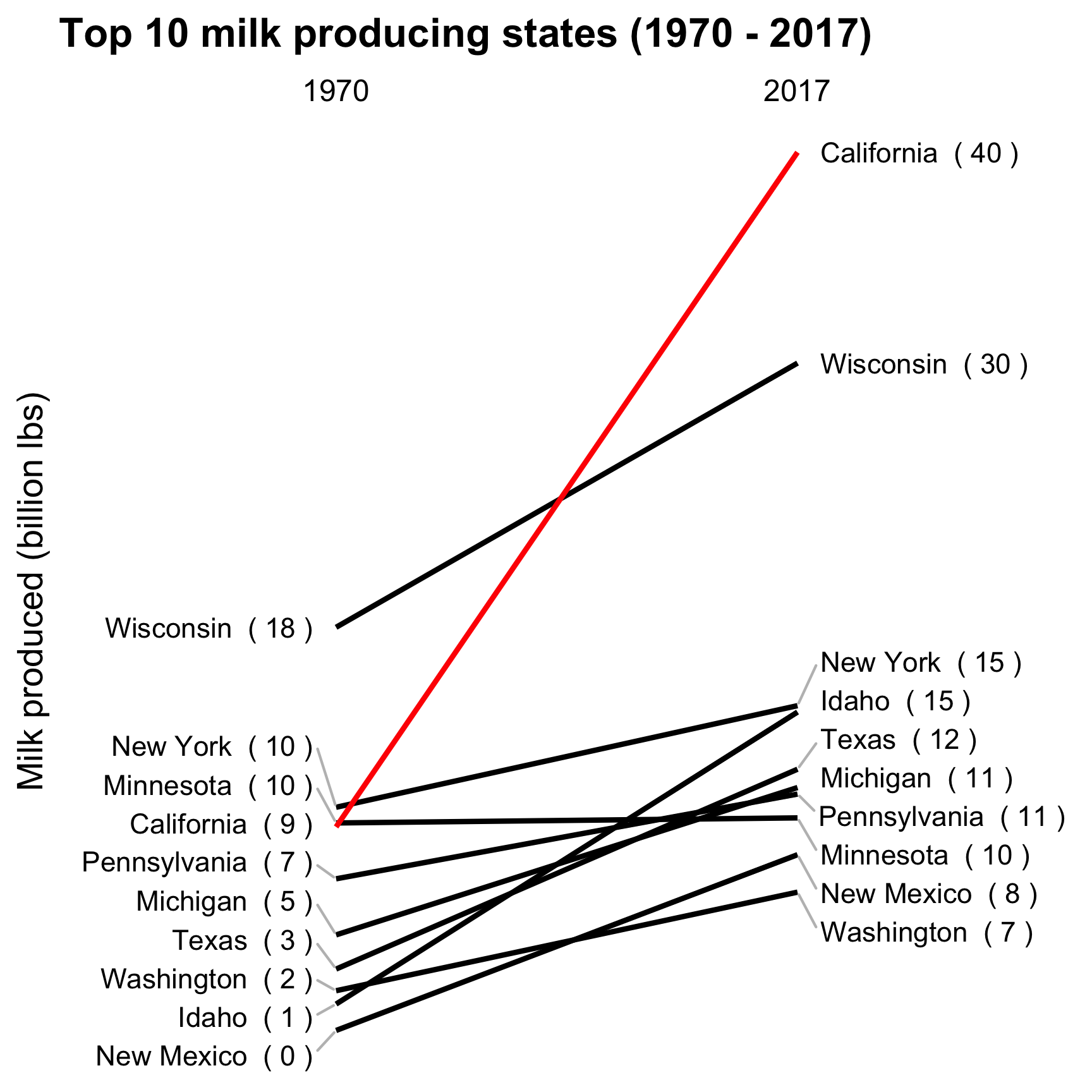
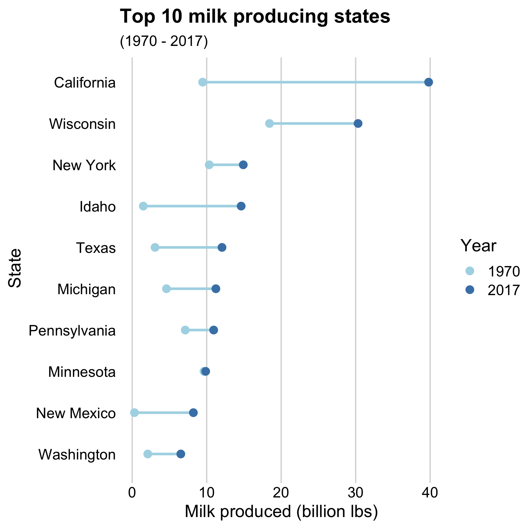
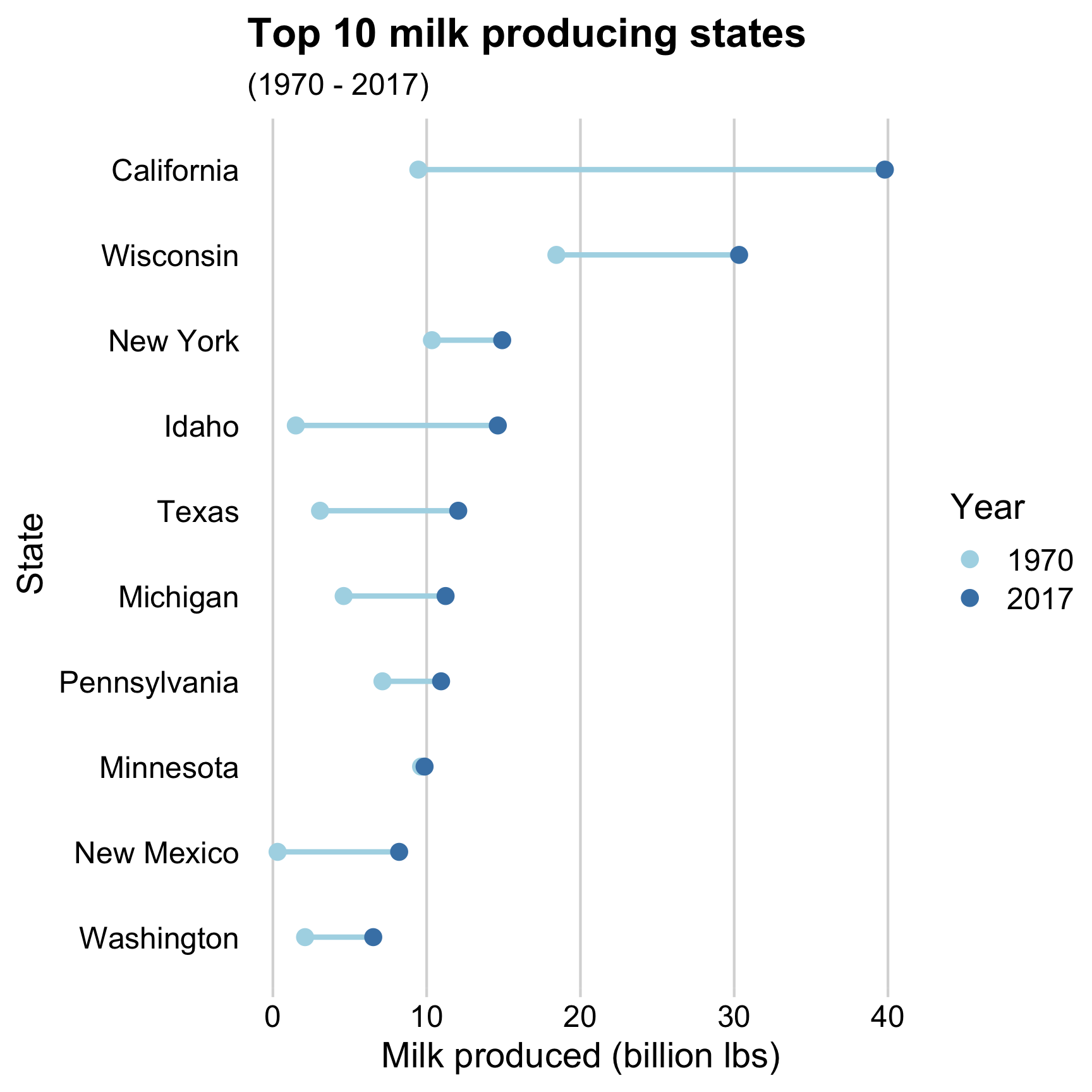
Dumbbell bars 😄
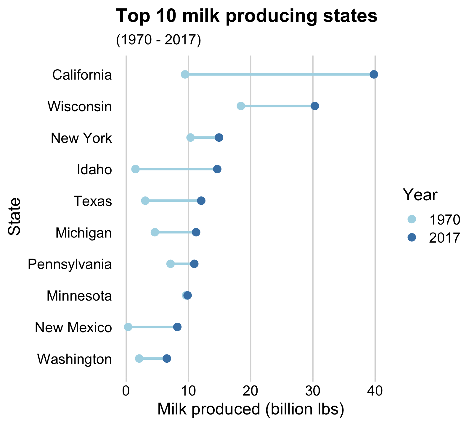
Strategies for comparing 2 things across more than 2 categories
Dodged bars 😢
Slope chart 😄
Dumbbell charts highlight:
- Compare magnitudes across two periods / groups
Slope charts highlight:
- Change in rankings
- Highlight individual categories
How to make a Dumbbell chart
Create data frame for plotting
top10states <- milk_production %>%
  filter(year == 2017) %>%
  arrange(desc(milk_produced)) %>%
  slice(1:10)

milk_summary_dumbbell <- milk_production %>%
  filter(
    year %in% c(1970, 2017),
    state %in% top10states$state
  ) %>%
  mutate(
    # Reorder state variables
    state = fct_reorder2(
      state,
      year,
      desc(milk_produced)
    ),
    # Convert year to discrete variable
    year = as.factor(year),
    # Modify units
    milk_produced = milk_produced / 10^9
  )
How to make a Dumbbell chart
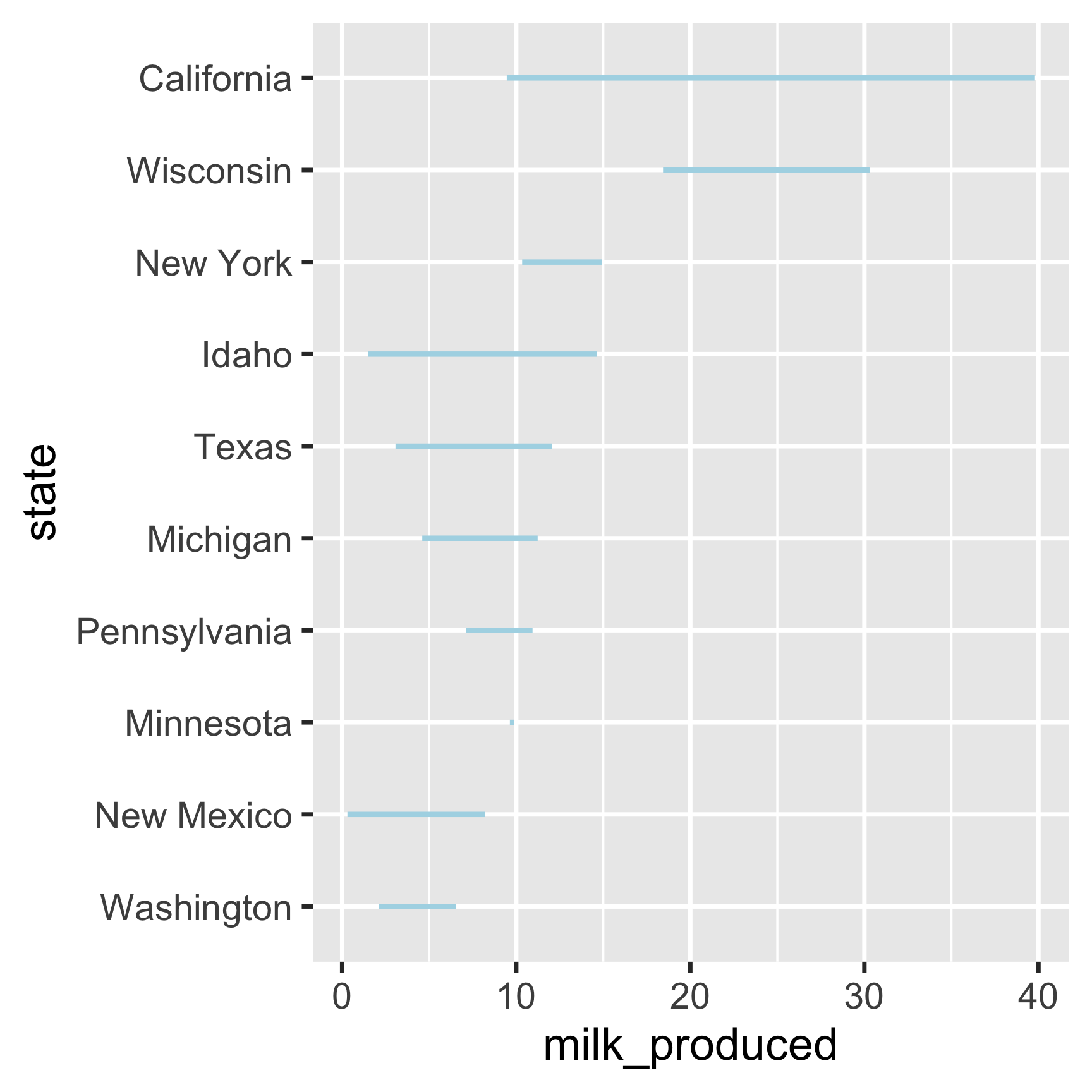
How to make a Dumbbell chart
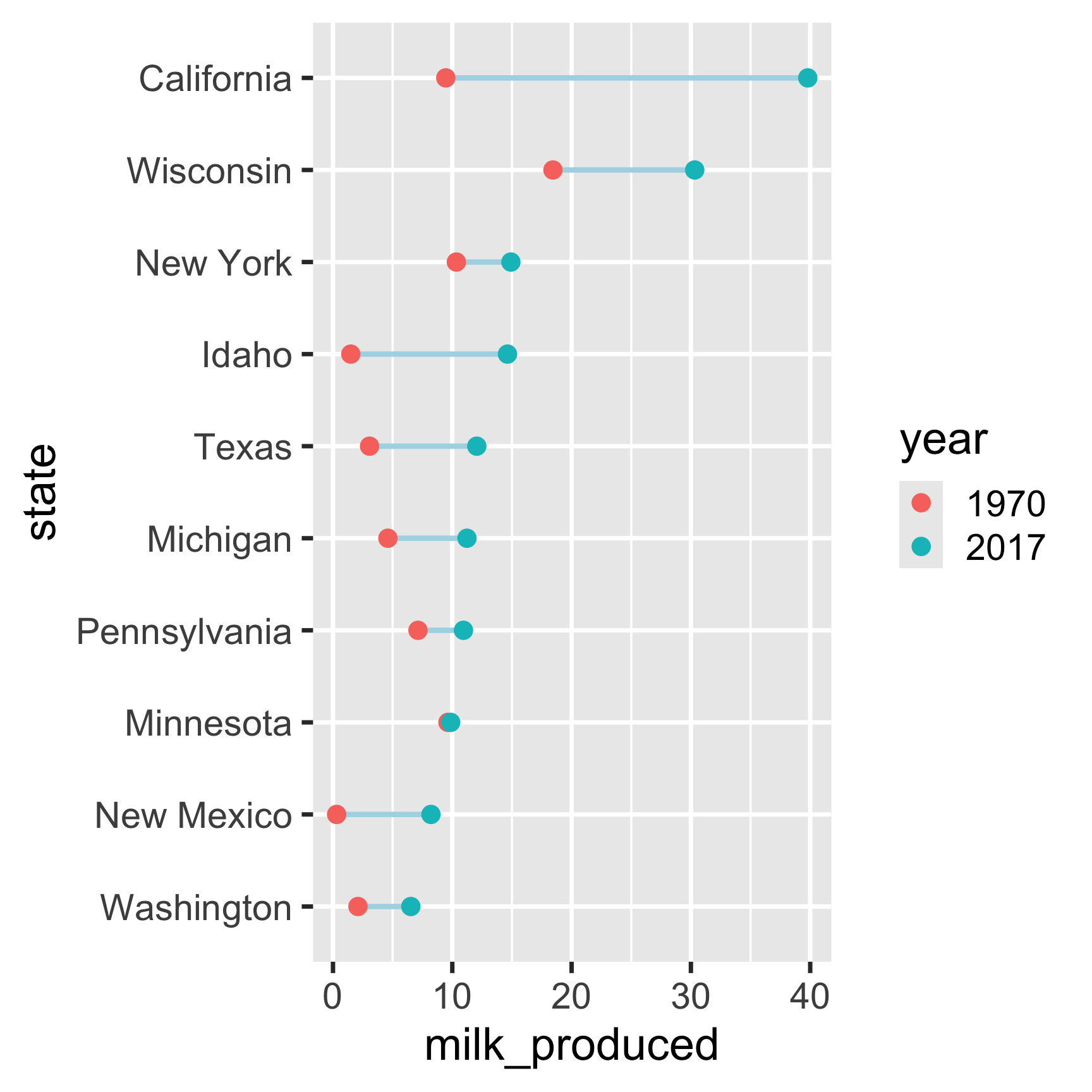
How to make a Dumbbell chart
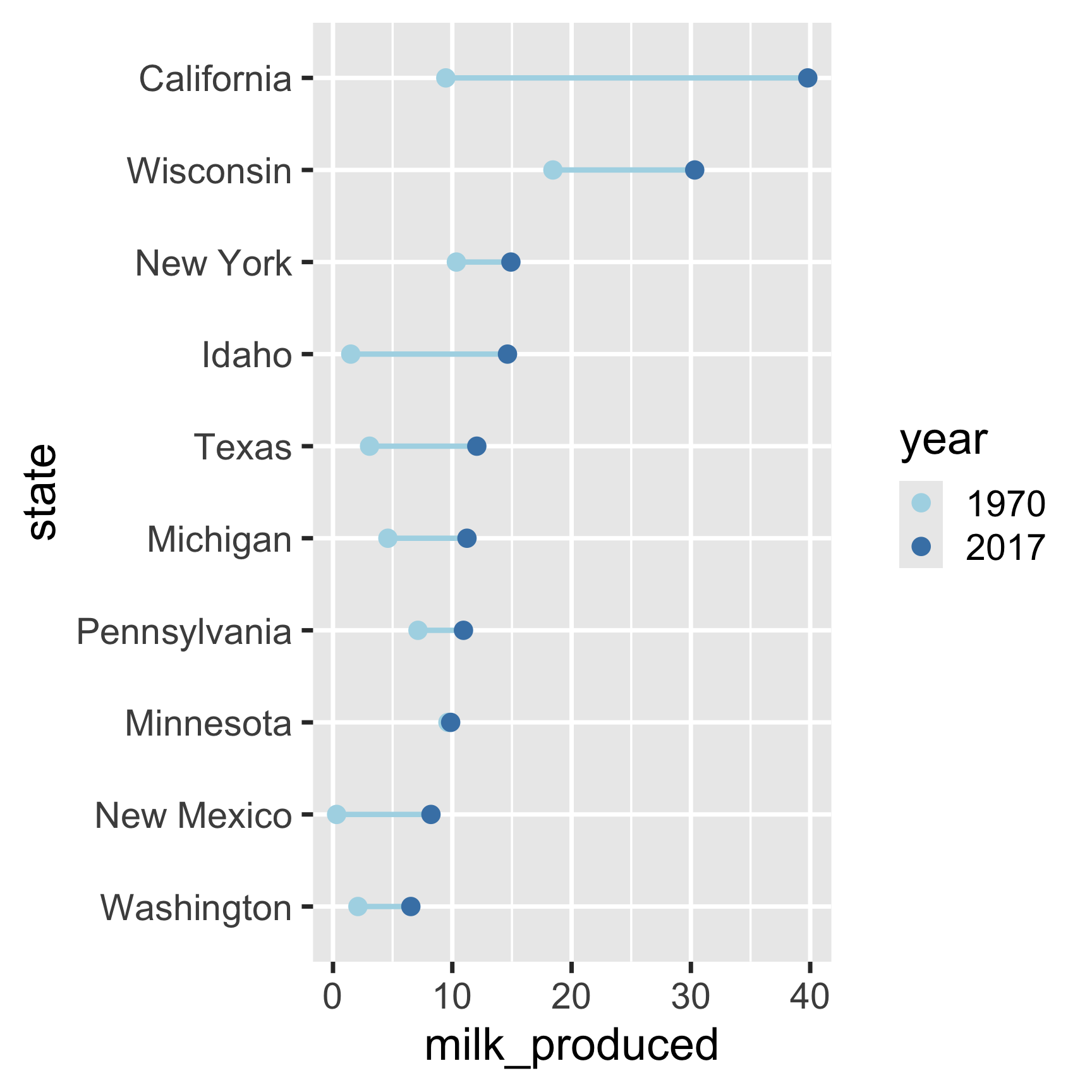
How to make a Dumbbell chart
Adjust the theme and annotate
ggplot(
     milk_summary_dumbbell,
     aes(x = milk_produced, y = state)
) +
     geom_line(
          aes(group = state),
          color = 'lightblue',
          size = 1
) +
geom_point(aes(color = year), size = 2.5) +
scale_color_manual(
values = c('lightblue', 'steelblue')
) +
theme_minimal_vgrid() +
# Remove y axis line and tick marks
theme(
axis.line.y = element_blank(),
axis.ticks.y = element_blank()
) +
labs(
x = 'Milk produced (billion lbs)',
y = 'State',
color = 'Year',
title = 'Top 10 milk producing states',
subtitle = '(1970 - 2017)'
)
Create data frame for plotting
top10states <- milk_production %>%
  filter(year == 2017) %>%
  arrange(desc(milk_produced)) %>%
  slice(1:10)

milk_summary_slope <- milk_production %>%
  filter(
    year %in% c(1970, 2017),
    state %in% top10states$state
  ) %>%
  mutate(
    # Reorder state variables
    state = fct_reorder2(state, year, desc(milk_produced)),
    # Convert year to discrete variable
    year = as.factor(year),
    # Modify units
    milk_produced = milk_produced / 10^9,
    # Define line color
    lineColor = if_else(
      state == 'California',
      'CA',
      'other'
    ),
    # Make labels
    label = paste(state, ' (', round(milk_produced), ')'),
    label_left = ifelse(year == 1970, label, NA),
    label_right = ifelse(year == 2017, label, NA)
  )
How to make a
Slope chart
Slope chart
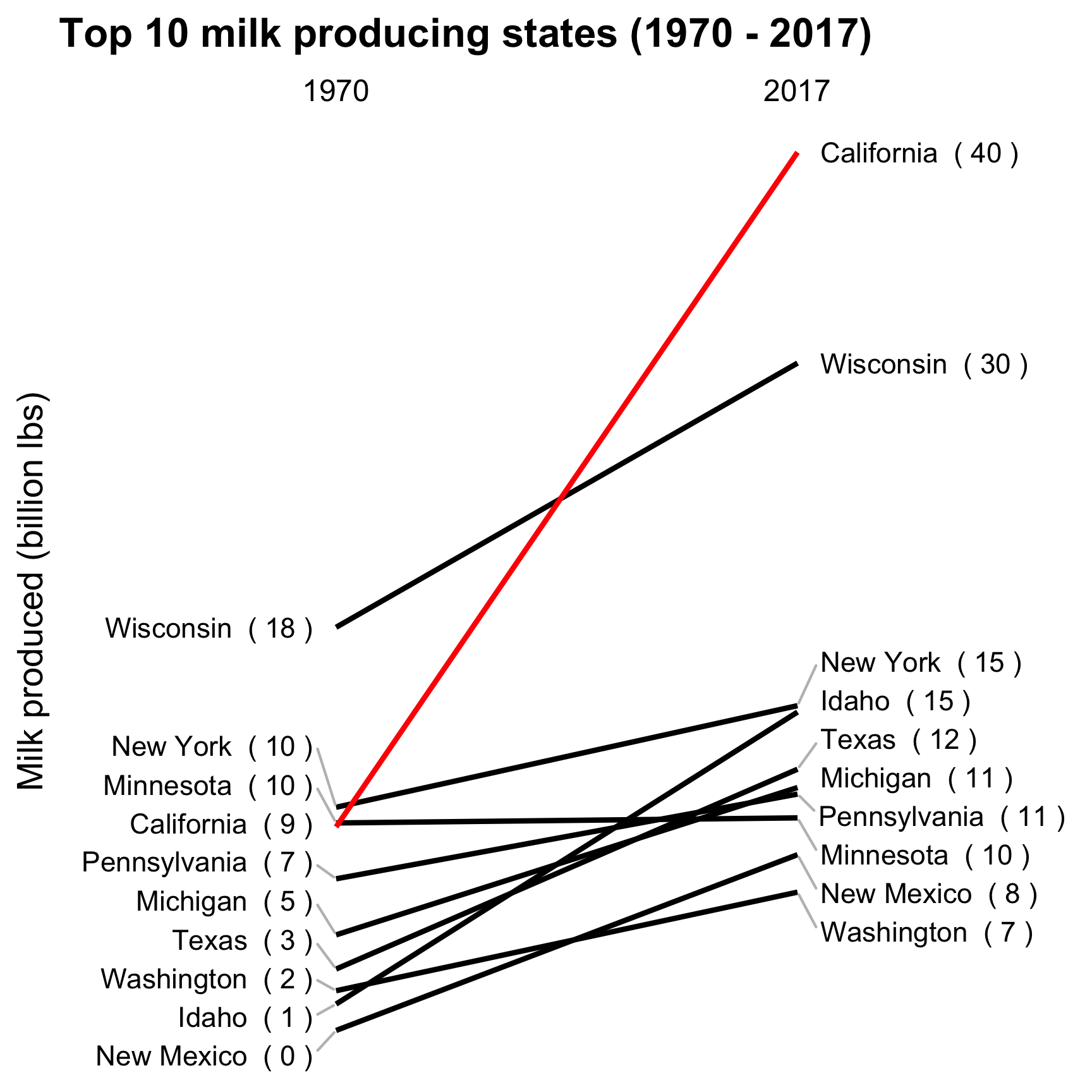
How to make a Slope chart
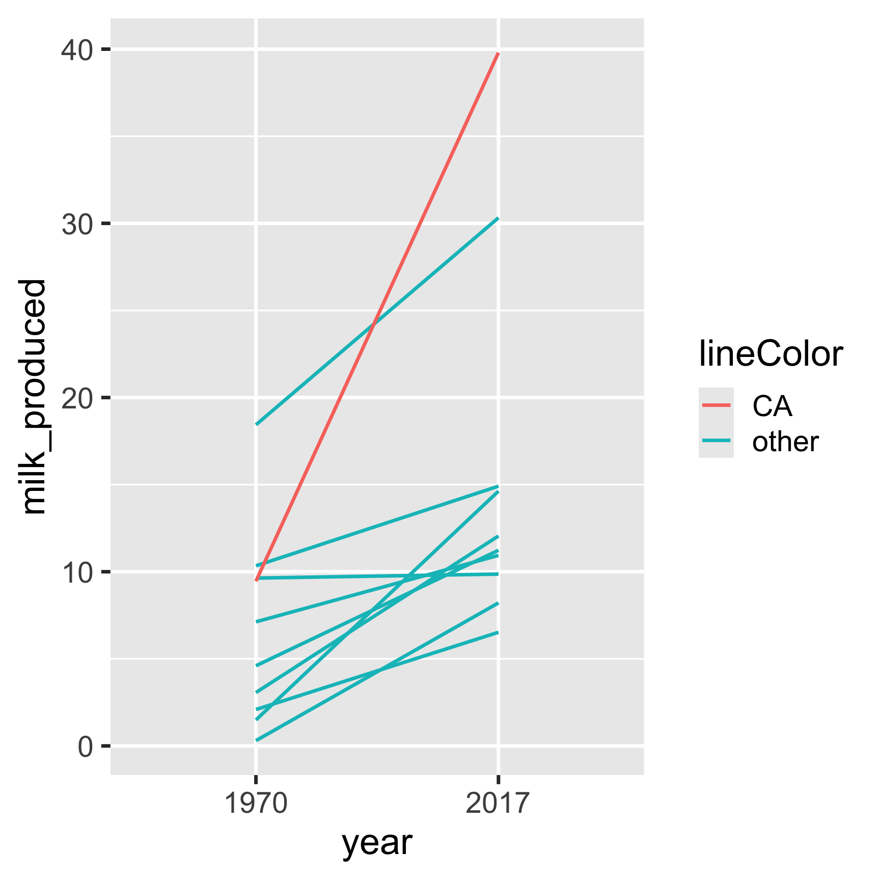
How to make a Slope chart
Add labels:
ggplot(
       milk_summary_slope,
       aes(x = year, y = milk_produced, group = state)
) +
geom_line(aes(color = lineColor)) +
# Add 1970 labels (left side)
geom_text(
aes(label = label_left),
hjust = 1,
nudge_x = -0.05
) +
# Add 2017 labels (right side)
geom_text(
aes(label = label_right),
hjust = 0,
nudge_x = 0.05
)| Justification | hjust |
|---|---|
| Left | 0 |
| Center | 0.5 |
| Right | 1 |
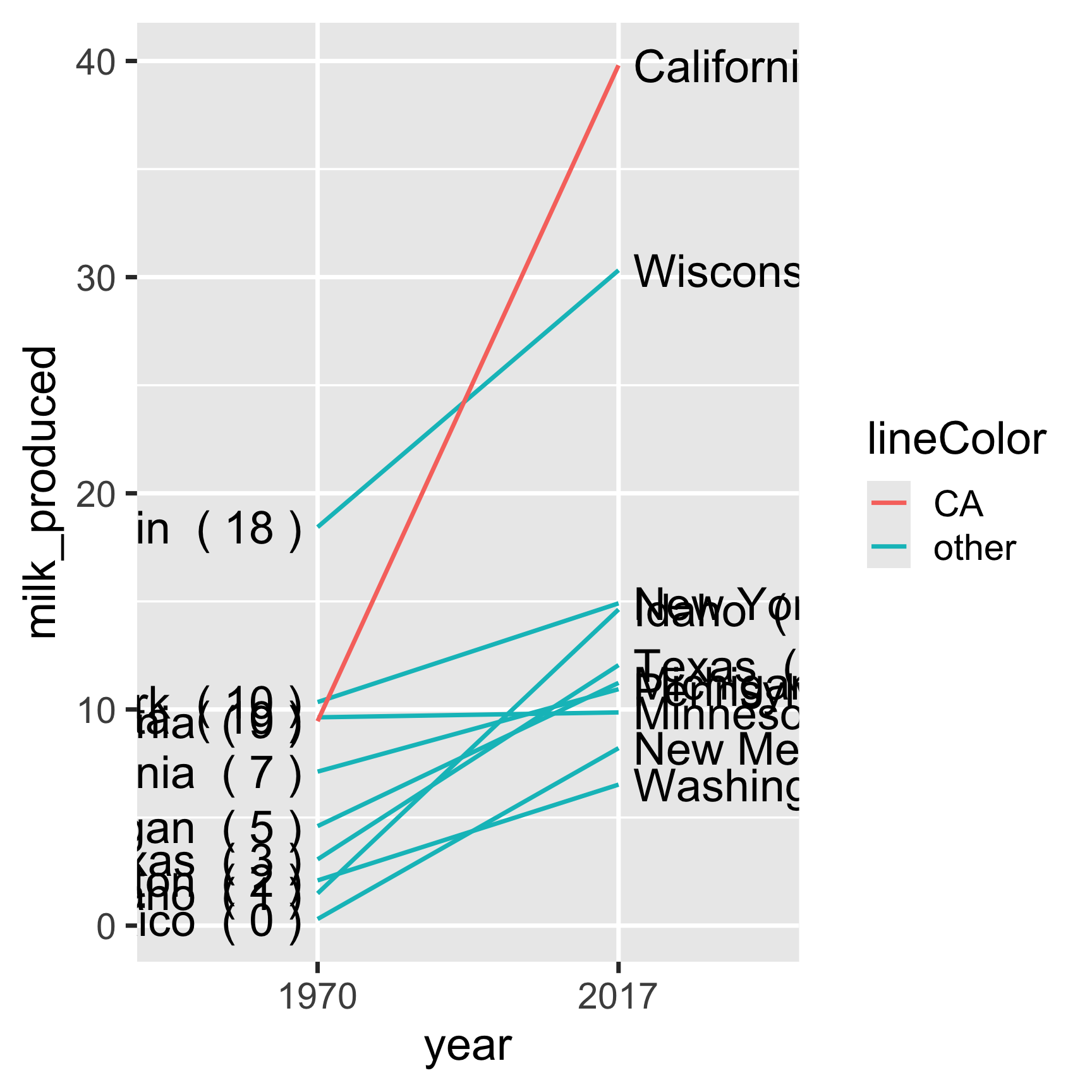
Overlapping labels?
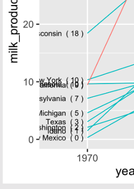
Overlapping labels?
ggrepel library to the rescue!
Artwork by @allison_horst
How to make a Slope chart
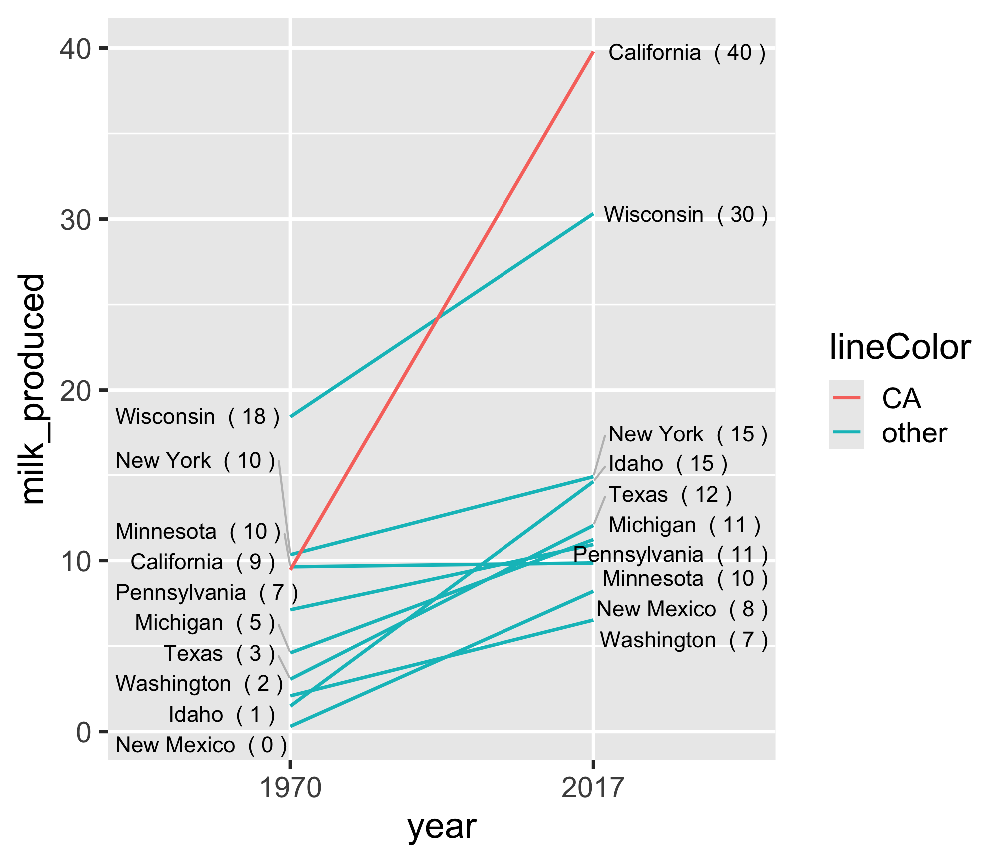
Align labels so they don’t overlap:
library(ggrepel)

ggplot(
  milk_summary_slope,
  aes(x = year, y = milk_produced, group = state)
) +
  geom_line(aes(color = lineColor)) +
  # Add 1970 labels (left side)
  geom_text_repel(
    aes(label = label_left),
    hjust = 1,
    nudge_x = -0.05,
    direction = 'y',
    segment.color = 'grey'
  ) +
  # Add 2017 labels (right side)
  geom_text_repel(
    aes(label = label_right),
    hjust = 0,
    nudge_x = 0.05,
    direction = 'y',
    segment.color = 'grey'
  )
How to make a Slope chart
Adjust colors:
ggplot(
  milk_summary_slope,
  aes(x = year, y = milk_produced, group = state)
) +
  geom_line(aes(color = lineColor)) +
  geom_text_repel(
    aes(label = label_left),
    hjust = 1,
    nudge_x = -0.05,
    direction = 'y',
    segment.color = 'grey'
  ) +
  geom_text_repel(
    aes(label = label_right),
    hjust = 0,
    nudge_x = 0.05,
    direction = 'y',
    segment.color = 'grey'
  ) +
  # Move year labels to top, modify line colors
  scale_x_discrete(position = 'top') +
  scale_color_manual(values = c('red', 'black'))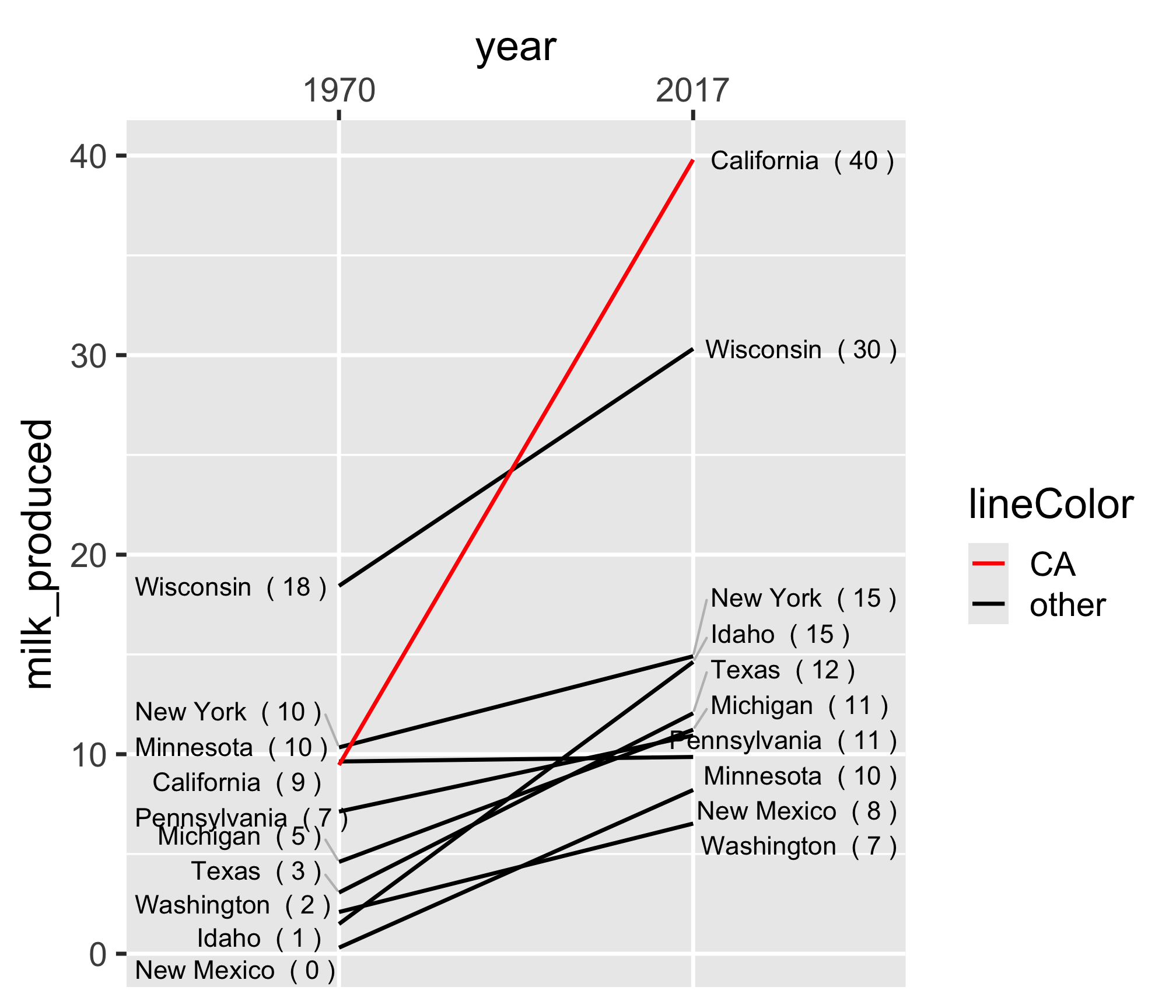
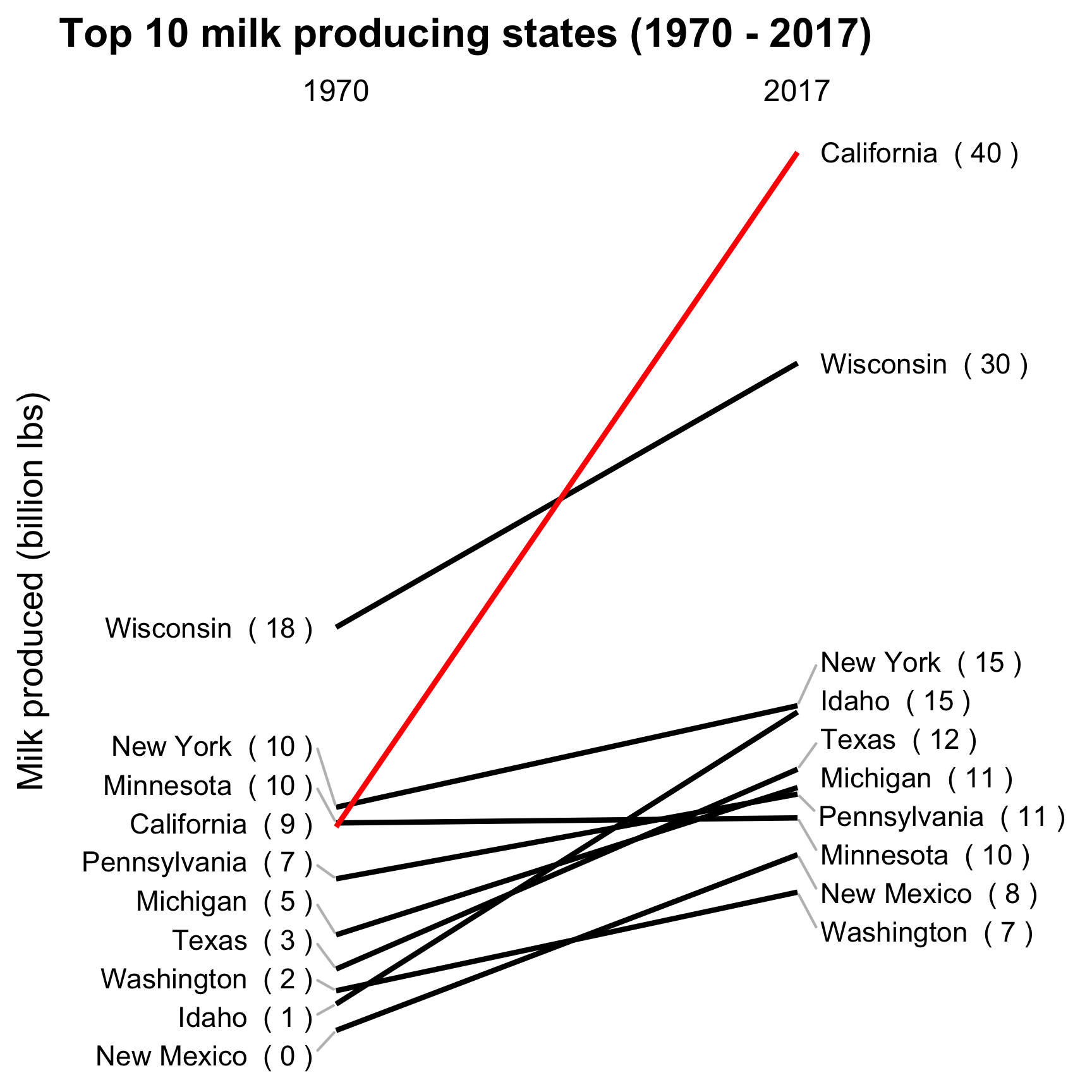
Adjust the theme and annotate
ggplot(
  milk_summary_slope,
  aes(x = year, y = milk_produced, group = state)
) +
  geom_line(aes(color = lineColor)) +
  # Add 1970 labels (left side)
  geom_text_repel(
    aes(label = label_left),
    hjust = 1,
    nudge_x = -0.05,
    direction = 'y',
    segment.color = 'grey'
  ) +
  # Add 2017 labels (right side)
  geom_text_repel(
    aes(label = label_right),
    hjust = 0,
    nudge_x = 0.05,
    direction = 'y',
    segment.color = 'grey'
  ) +
  # Move year labels to top, modify line colors
  scale_x_discrete(position = 'top') +
  scale_color_manual(values = c('red', 'black')) +
  # Annotate & adjust theme
  labs(
    x = NULL,
    y = 'Milk produced (billion lbs)',
    title = 'Top 10 milk producing states (1970 - 2017)'
  ) +
  theme_minimal_grid() +
  theme(
    panel.grid = element_blank(),
    axis.text.y = element_blank(),
    axis.ticks = element_blank(),
    legend.position = 'none'
  )
How to make a
Slope chart
Slope chart
20:00
Your turn - comparing multiple categories
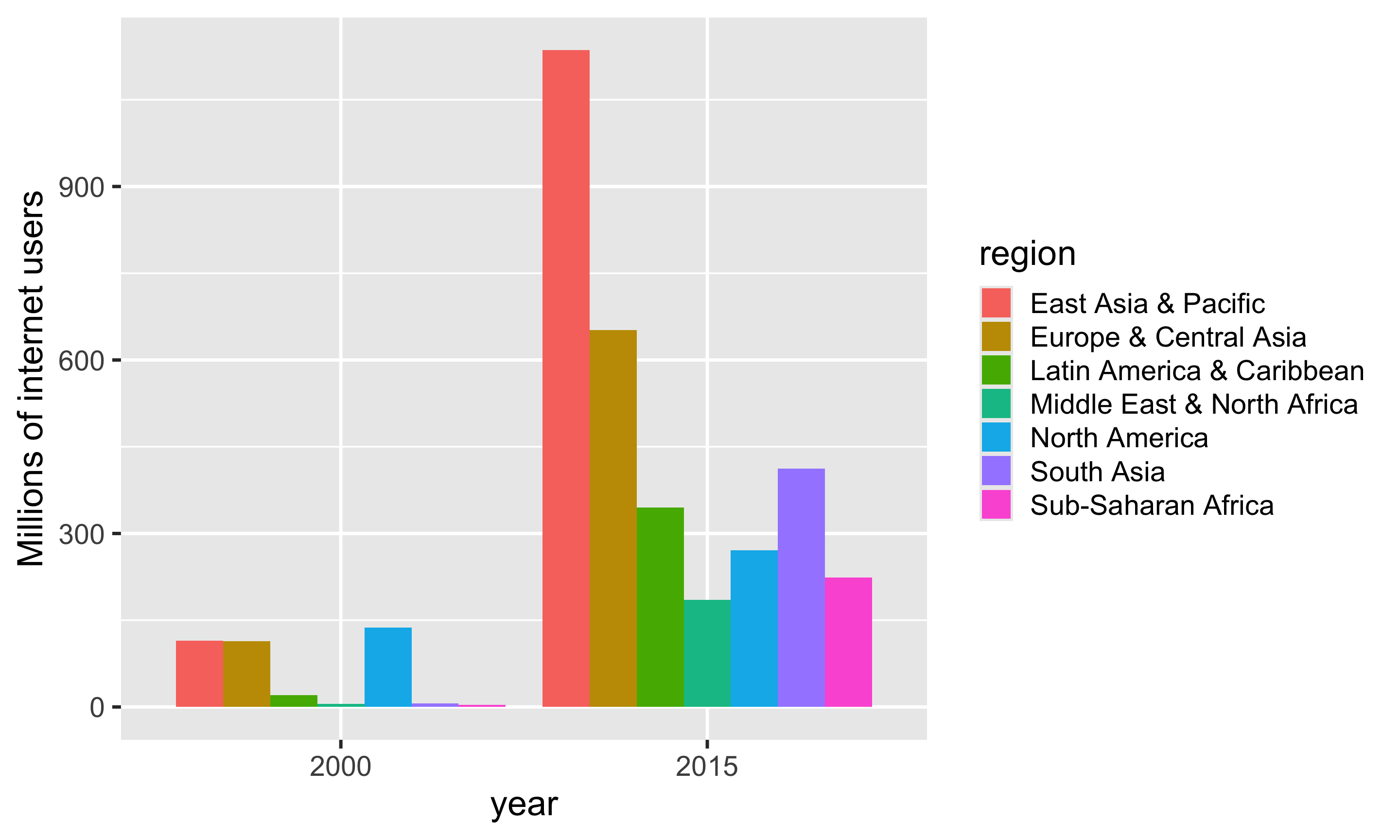
Using the internet_regions data frame, pick a strategy and create an improved version of this chart.
Strategies:
- Dodged bars
- Facets
- Bullet chart
- Dumbell chart
- Slope chart
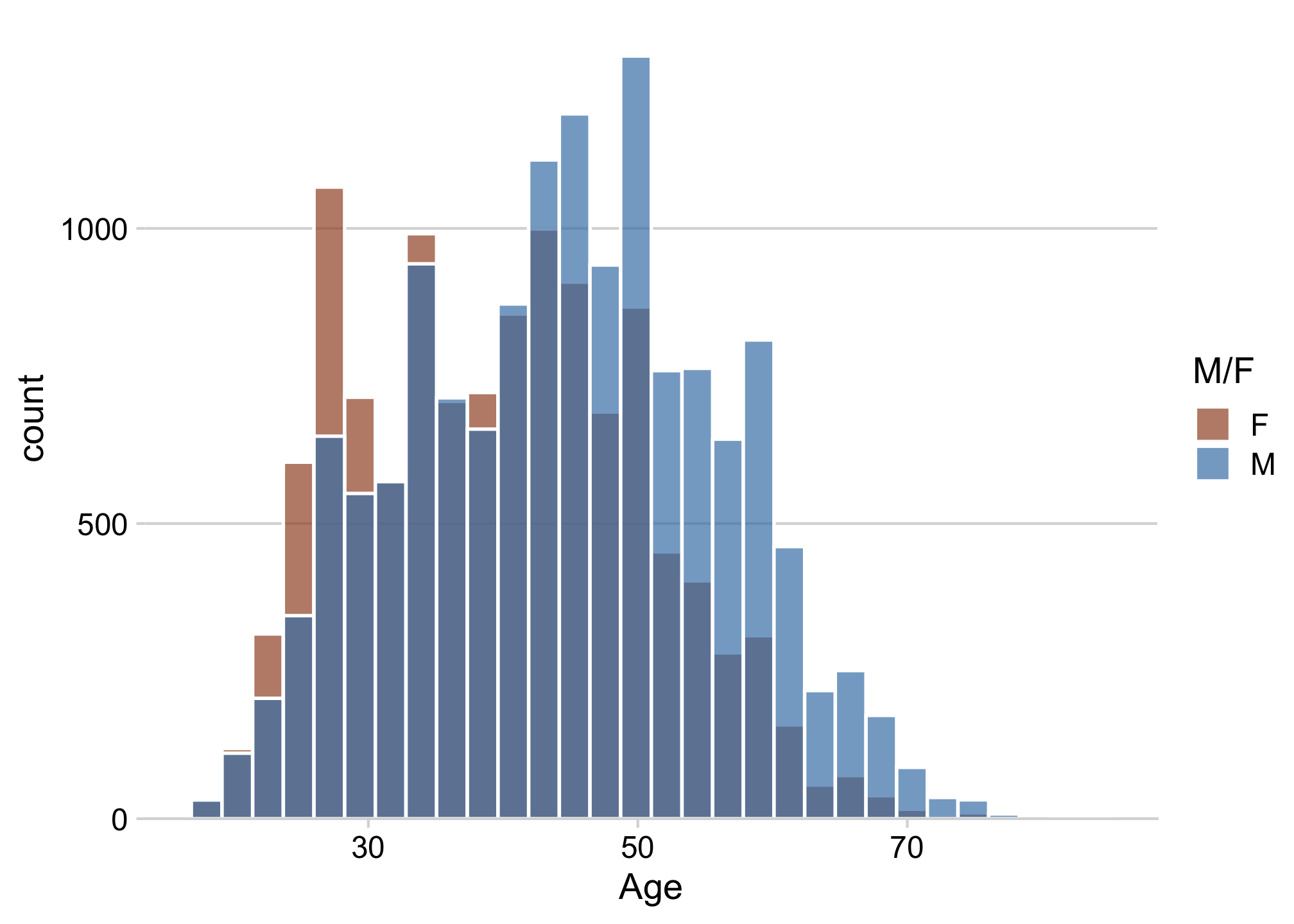
Overlapping histograms have issues
Bad
Slightly better
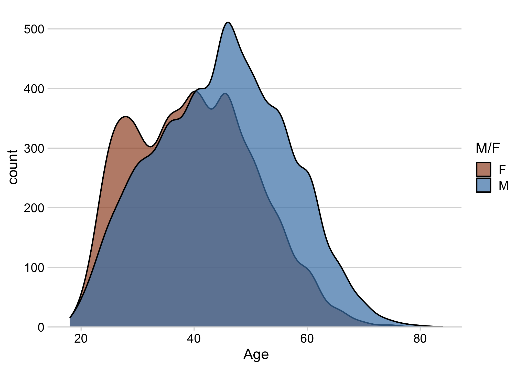
Good when number of categories is small
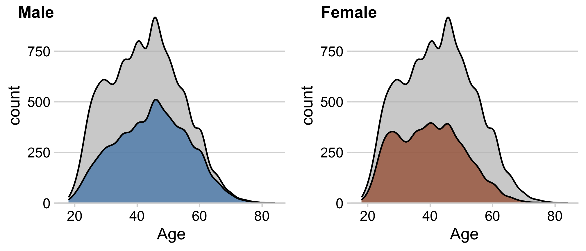
Density facets
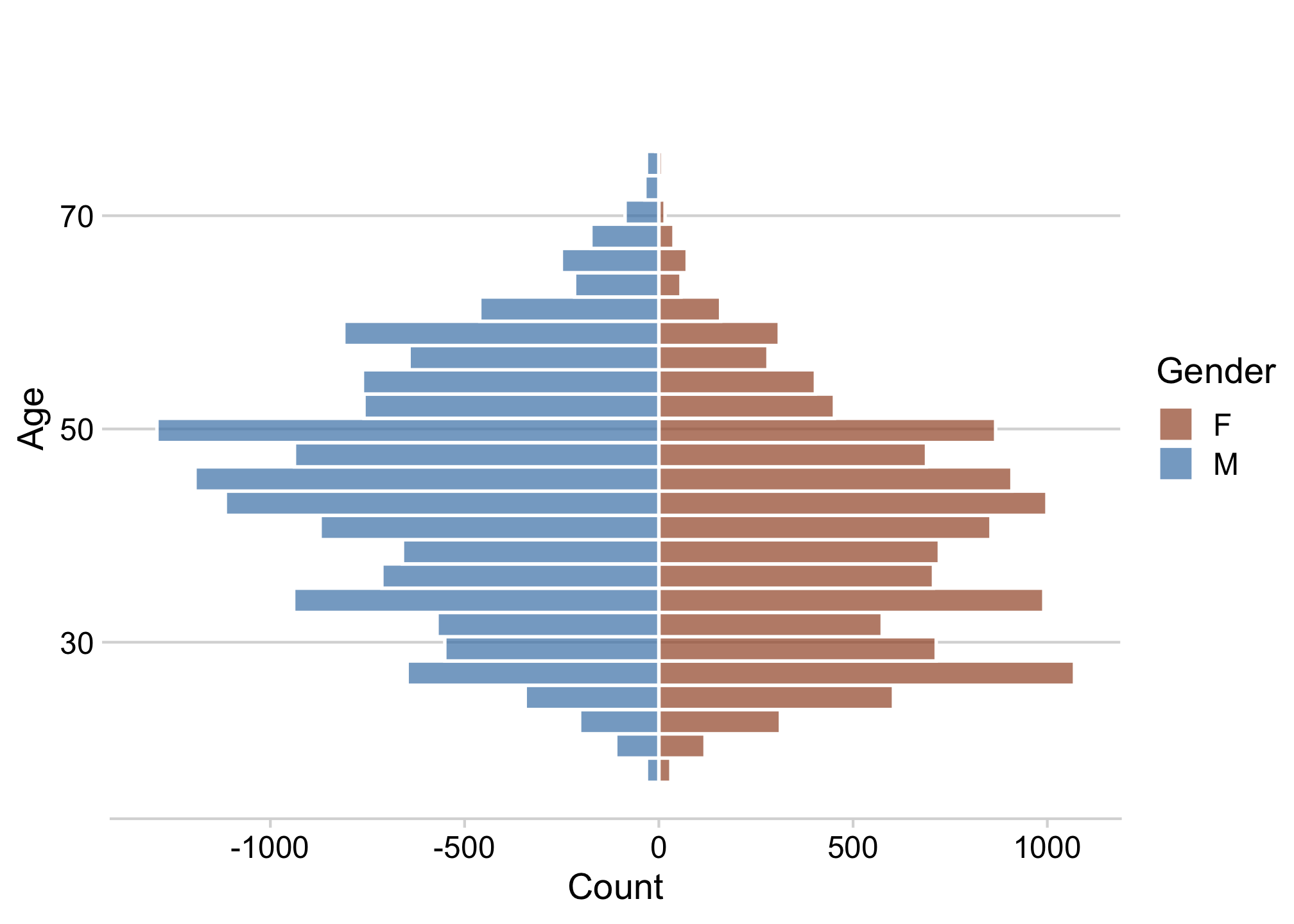
Diverging histograms
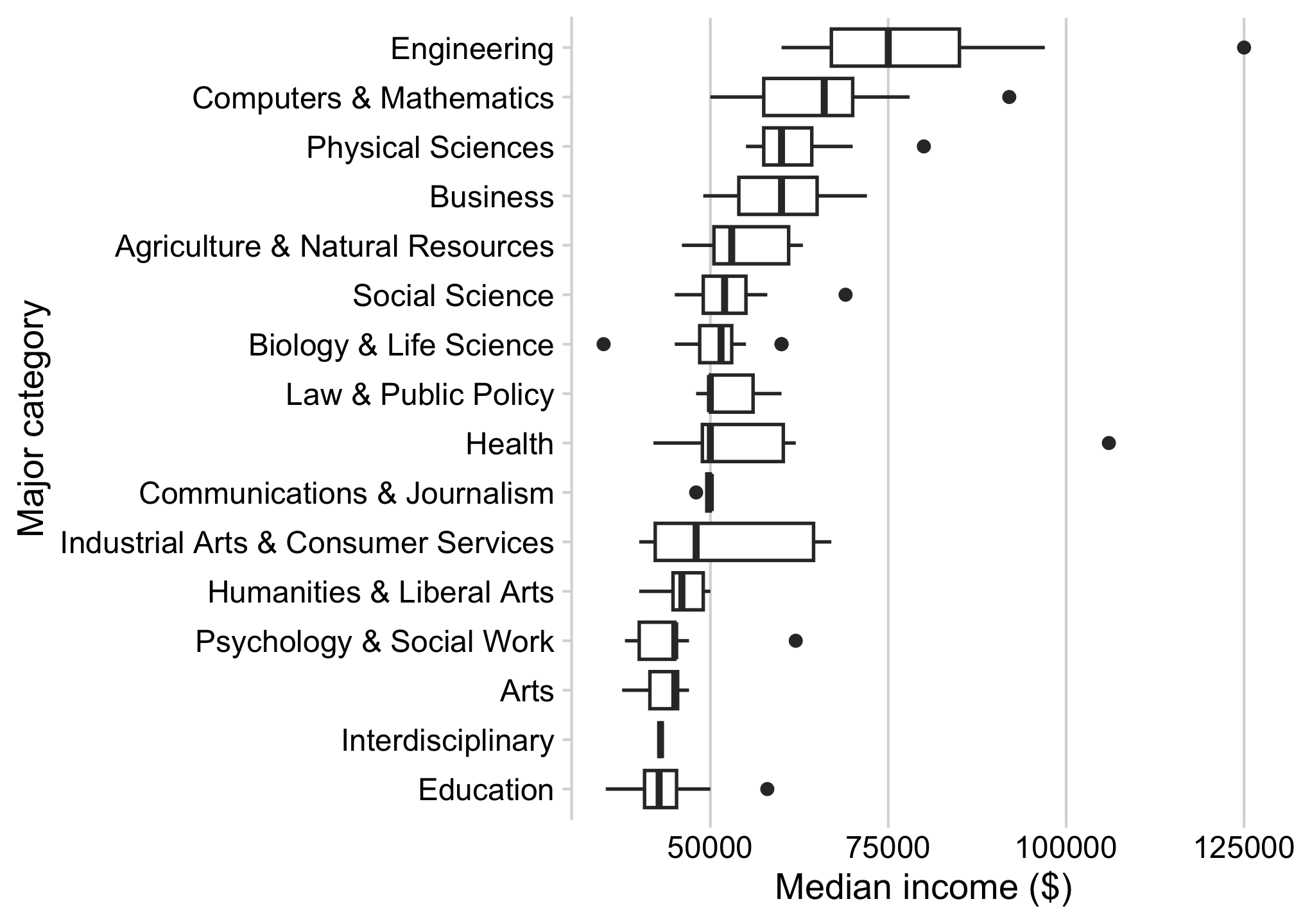
Good when number of categories is large
Boxplot
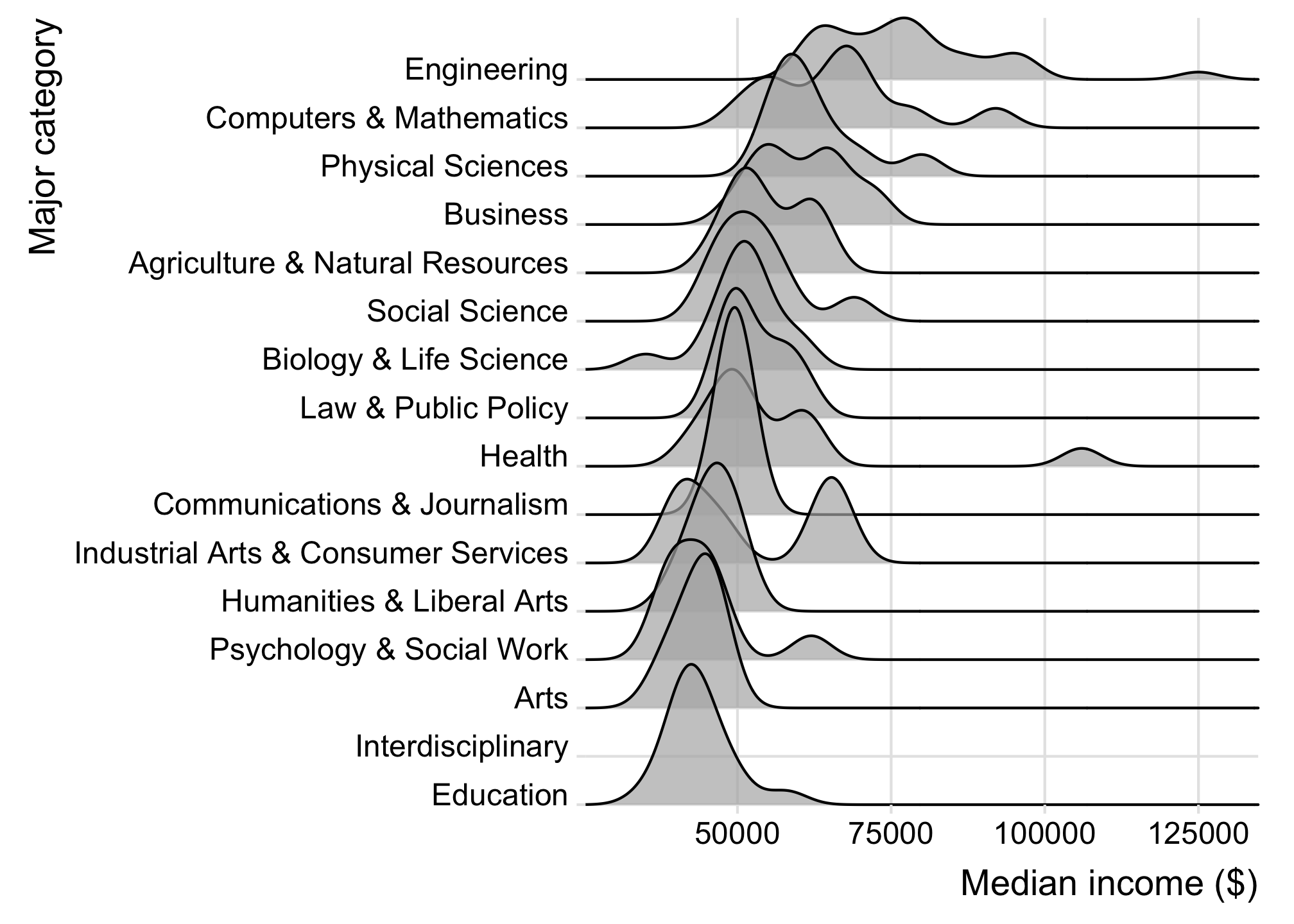
Ridgeplot
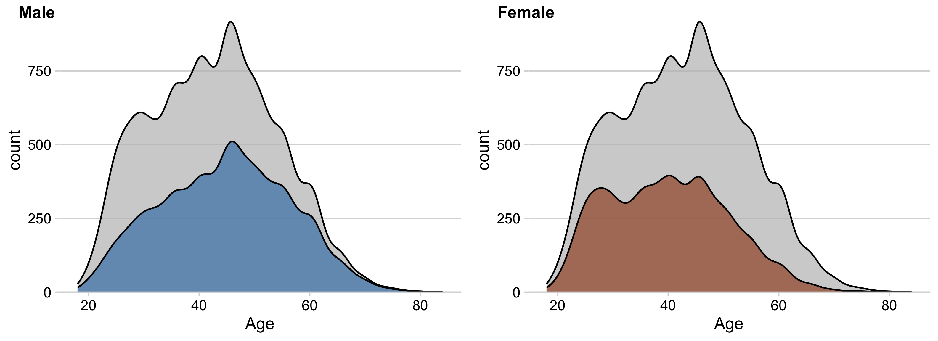
How to make density facets
You can use facet_wrap(), but
you won’t get the full density overlay
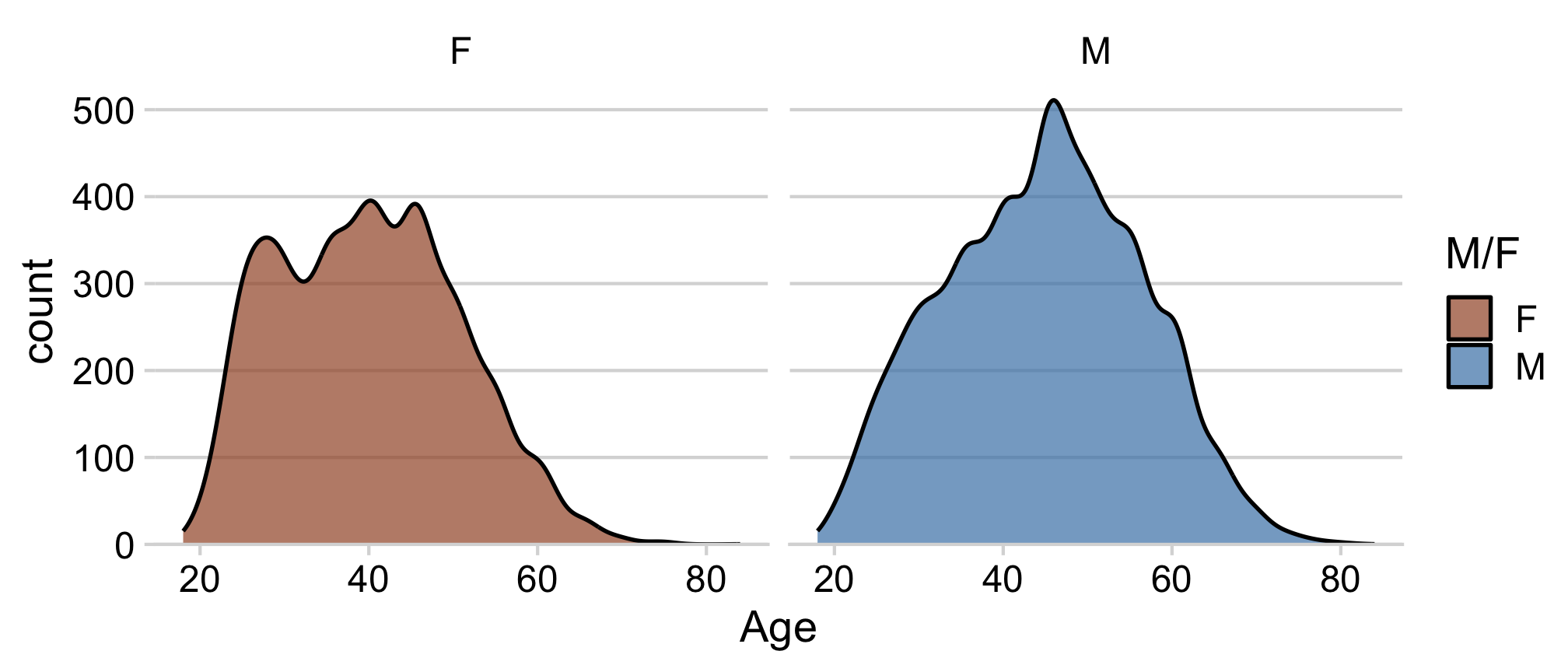
If you want the full density overlay,
you have to hand-make the facets
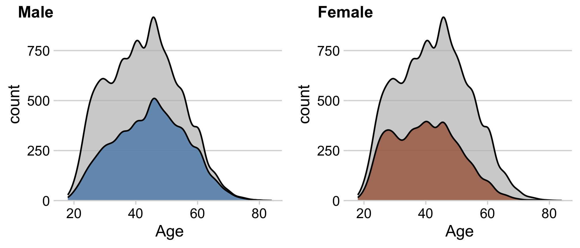
How to make density facets
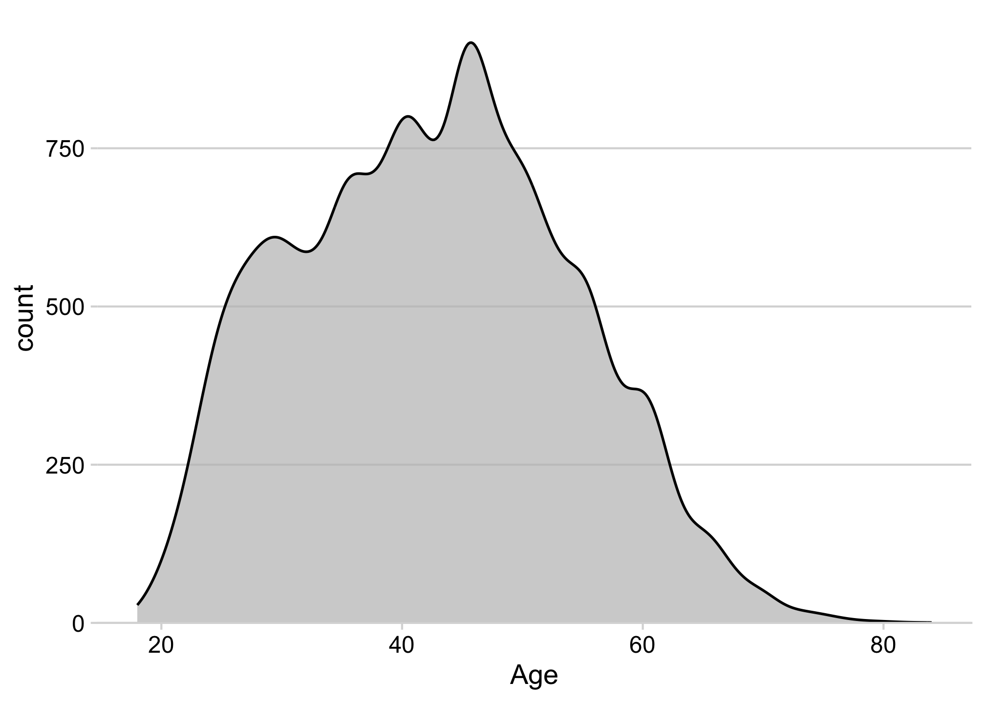
How to make density facets
Separately create each sub-plot
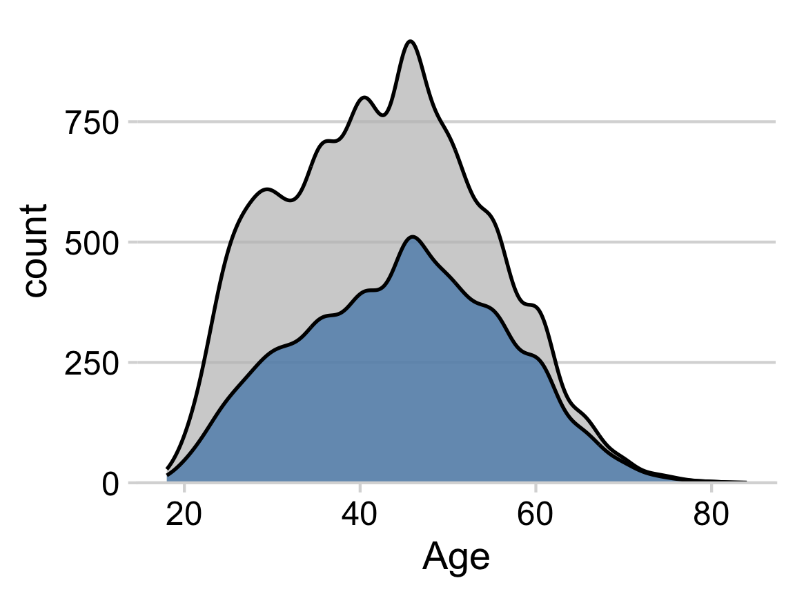
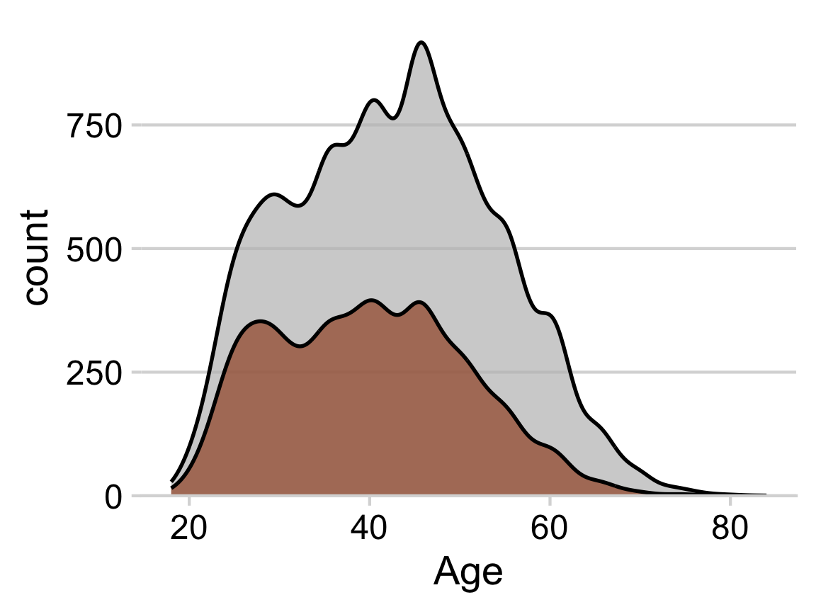
How to make density facets
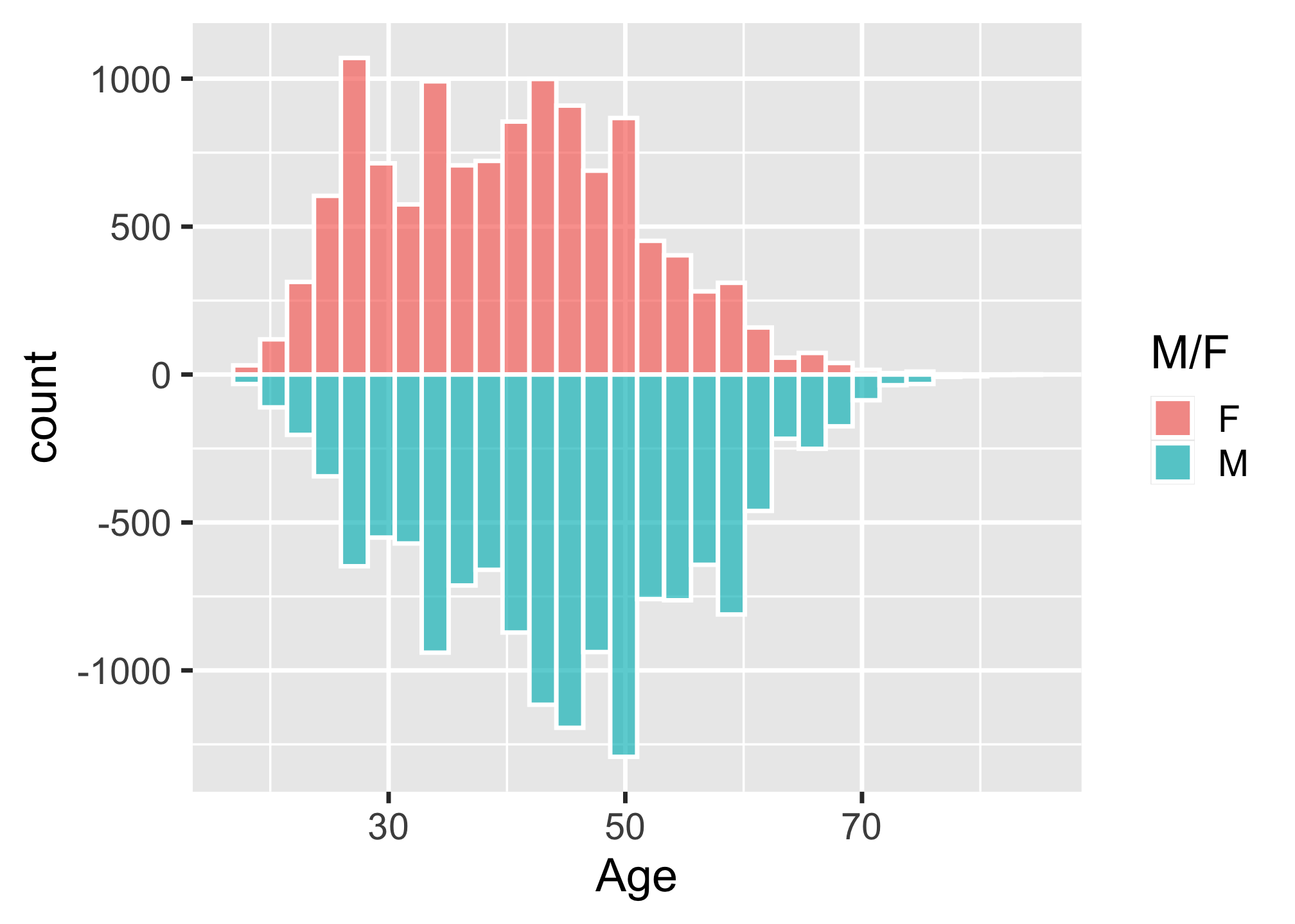
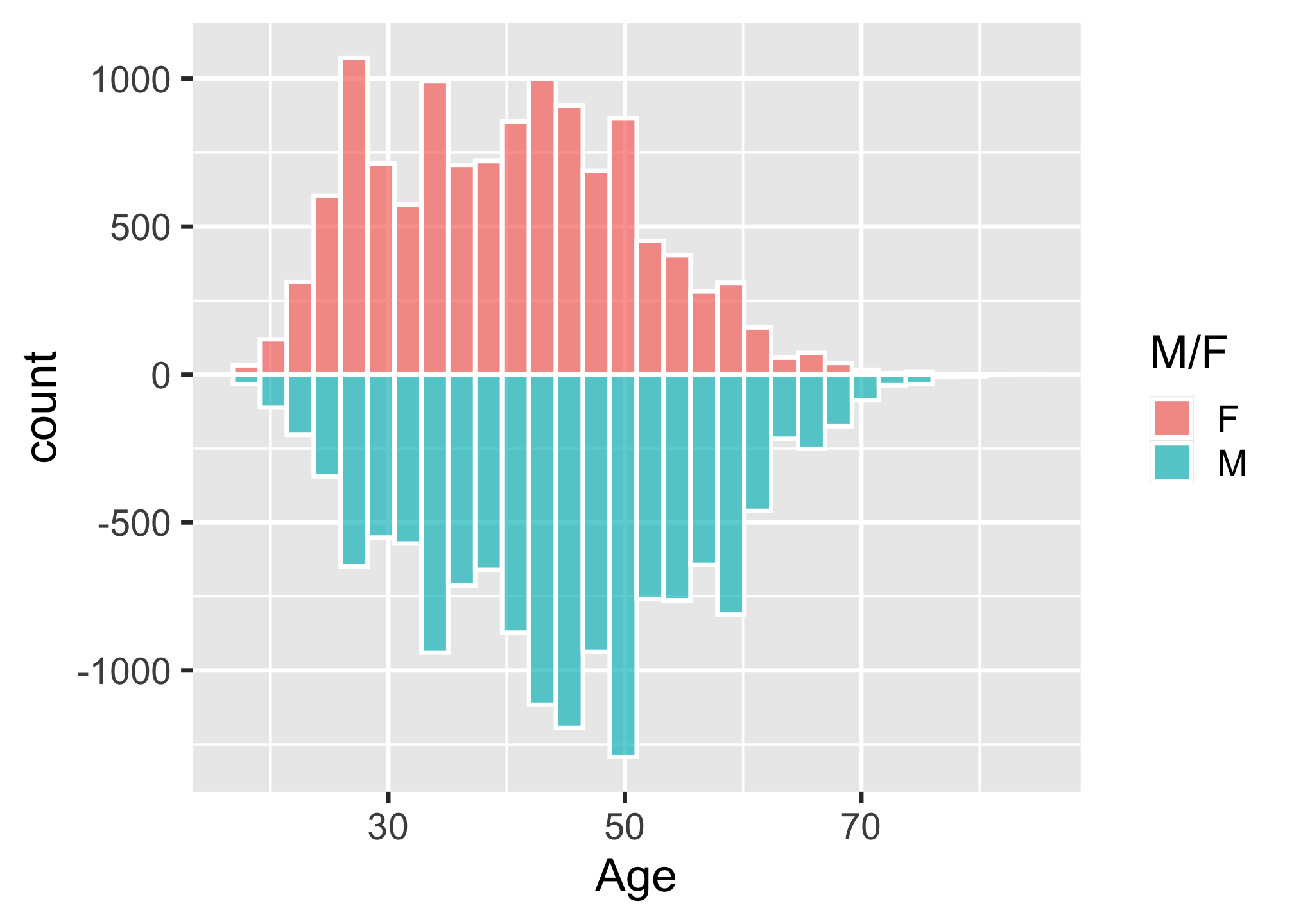
How to make diverging histograms
Make the histograms by filtering the data
ggplot(marathon, aes(x = Age)) +
  # Add histogram for Female runners:
  geom_histogram(
    data = marathon %>%
      filter(`M/F` == 'F'),
    aes(fill = `M/F`, y = ..count..),
    alpha = 0.7,
    color = 'white'
  ) +
  # Add negative histogram for Male runners:
  geom_histogram(
    data = marathon %>%
      filter(`M/F` == 'M'),
    aes(fill = `M/F`, y = ..count.. * (-1)),
    alpha = 0.7,
    color = 'white'
  )
How to make diverging histograms
Make the histograms by filtering the data
ggplot(marathon, aes(x = Age)) +
  # Add histogram for Female runners:
  geom_histogram(
    data = marathon %>%
      filter(`M/F` == 'F'),
    aes(fill = `M/F`, y = ..count..),
    alpha = 0.7,
    color = 'white'
  ) +
  # Add negative histogram for Male runners:
  geom_histogram(
    data = marathon %>%
      filter(`M/F` == 'M'),
    aes(fill = `M/F`, y = ..count.. * (-1)),
    alpha = 0.7,
    color = 'white'
  )
How to make diverging histograms
Rotate, adjust colors, theme, annotate
ggplot(marathon, aes(x = Age)) +
  # Add histogram for Female runners:
  geom_histogram(
    data = marathon %>%
      filter(`M/F` == 'F'),
    aes(fill = `M/F`, y = ..count..),
    alpha = 0.7,
    color = 'white'
  ) +
  # Add negative histogram for Male runners:
  geom_histogram(
    data = marathon %>%
      filter(`M/F` == 'M'),
    aes(fill = `M/F`, y = ..count.. * (-1)),
    alpha = 0.7,
    color = 'white'
  ) +
  scale_fill_manual(
    values = c('sienna', 'steelblue')
  ) +
  coord_flip() +
  theme_minimal_hgrid() +
  labs(fill = 'Gender', y = 'Count')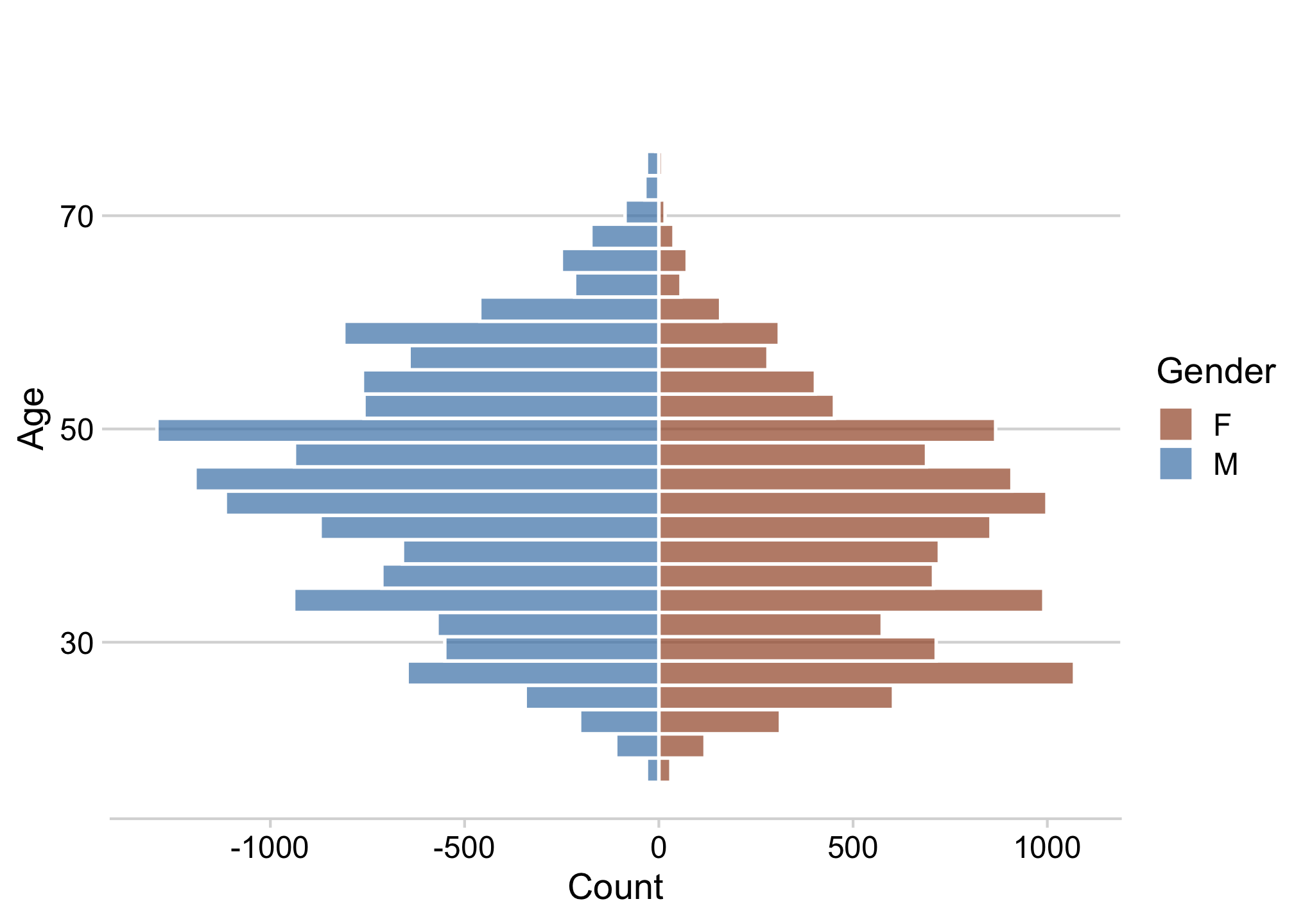
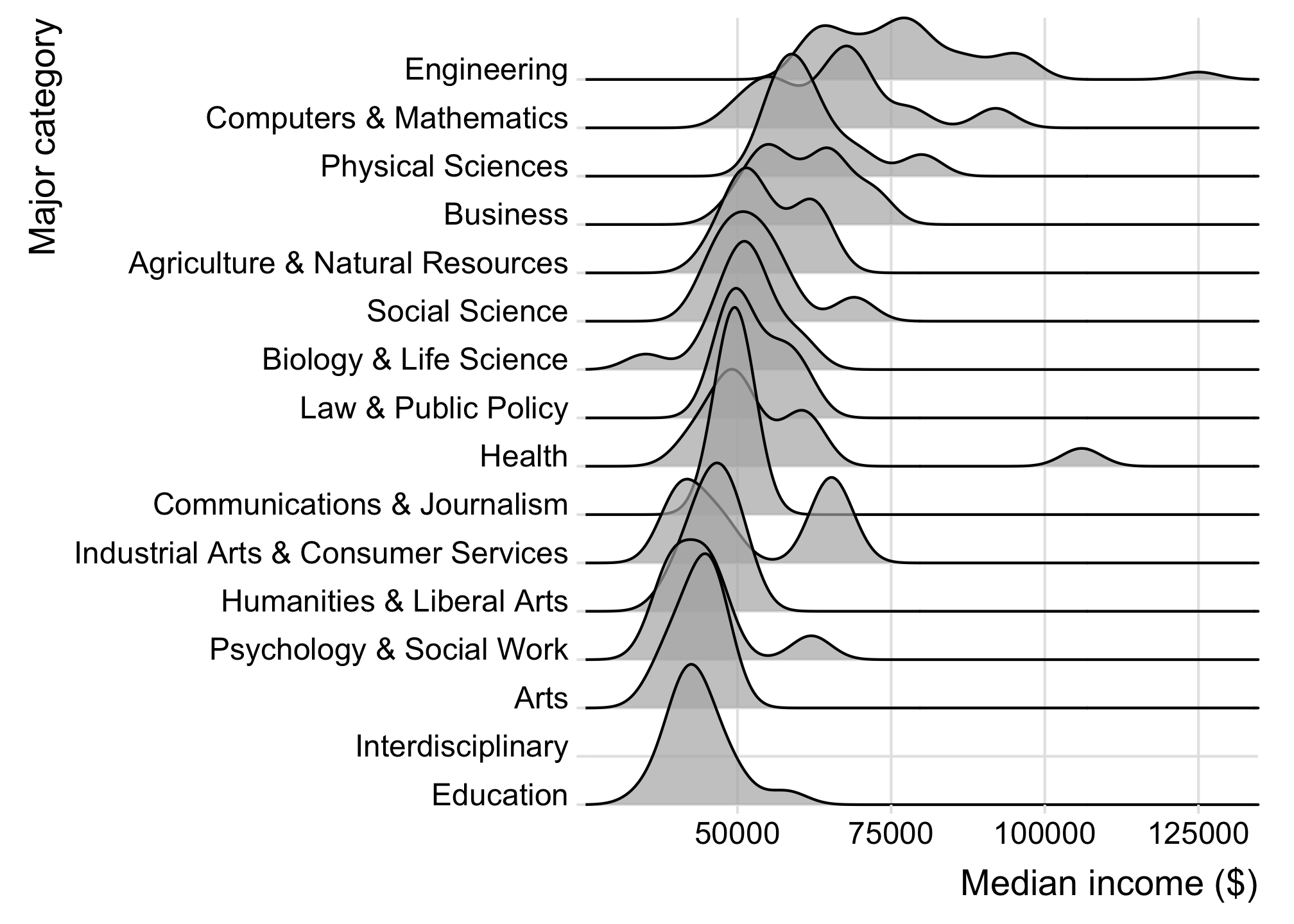
How to make ridgeplots
Make a ridgeplot with ggridges library
library(ggridges)

college_all_ages %>%
  mutate(
    major_category = fct_reorder(
      major_category,
      median
    )
  ) %>%
  ggplot() +
  geom_density_ridges(
    aes(x = median, y = major_category),
    scale = 4,
    alpha = 0.7
  ) +
  scale_y_discrete(expand = c(0, 0)) +
  scale_x_continuous(expand = c(0, 0)) +
  coord_cartesian(clip = "off") +
  theme_ridges() +
  labs(
    x = 'Median income ($)',
    y = 'Major category'
  )
15:00
Your turn - comparing distributions
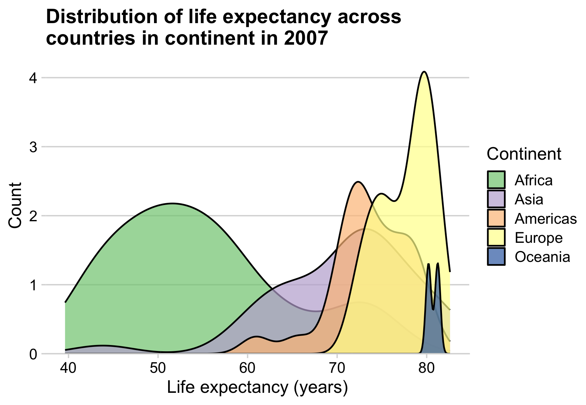
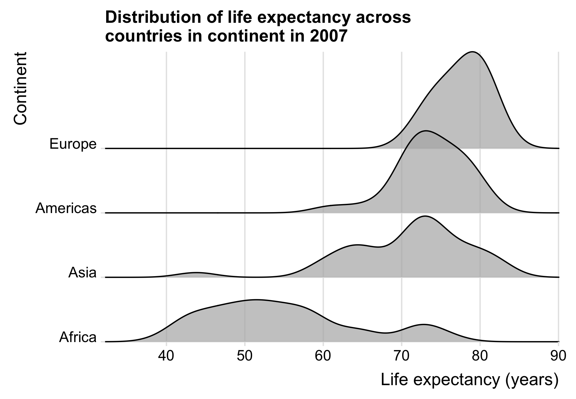
Use the gapminder.csv data to create the following charts comparing the distribution of life expectancy across countries in continents in 2007.