Data source by WEForum (2023), originated from BCSE.
This simple statistic emphasizes the growing prominence of renewable energy in the US, which is likely not to slow down anytime soon as renewables have the fastest growth rate of all energy sources at 12.6% (BCSE). This growth has been rapid: the contribution of renewables has almost doubled in just one decade (BCSE). The urgency of the climate crisis is the likely instigator of not only the United State’s renewable energy transition but also the global growth of renewables. The United States is a global renewable energy leader, ranking as the second highest producer of solar and wind energy in 2021 (IRENA).
Code
# 1. Load and clean data of international solar and wind gendrop <-c('World', 'Asia', 'Europe', 'North America','European Union', 'South America', 'Eurasia', 'Africa')internationalPath <-here('data', 'irena_solar_wind_international_raw.csv')international <-read_csv(internationalPath, skip =2) %>%rename(Country ='Region/country/area') %>%pivot_longer(names_to ='Year',values_to ='Generation',cols ='2000':'2021') %>%mutate(Year =as.numeric(Year) ) %>%filter(!Country %in% drop)international %>%write_csv(here('data', 'irena_solar_wind_international_long.csv'))# 2. International Solar Generation# 2.1 Solar gen data framesolar_international <- international %>%filter(Technology =='Solar')# 2.2 Top 5 solar producers in 2021top_5_solar <- solar_international %>%filter(Year =='2021') %>%arrange(desc(Generation)) %>%slice(1:5)# 2.3 Plot of top 5 solar producerssolar_international_plot <-ggplot(solar_international %>%filter(Country %in%c(top_5_solar$Country)),aes(x = Year, y = Generation/1000, group = Country, color = Country)) +geom_line(linewidth =1) +geom_text_repel(data = top_5_solar,aes(label = Country),hjust =0, nudge_x =1, direction ="y",size =5, segment.color =NA,family ="Ubuntu") +scale_x_continuous(breaks =seq(2000, 2021, 3),expand =expansion(add =c(1, 5))) +scale_y_continuous(expand =expand_scale(mult =c(0, 0.05))) +labs(x ='Year',y ='Generation (TWh)',title ='United States is the second highest producer of\nsolar energy',subtitle ='Top 5 producers of solar energy in 2021',caption ='Data from IRENA') +scale_color_manual(values =c('#719847','#ccca5d','#b2529d','#4c67a5','#a5734c')) +theme_minimal_hgrid(font_family ='Ubuntu') +theme(legend.position ='none')ggsave(filename =here('figs_manu', '3_1_solar_inter_plot.png'), plot = solar_international_plot,width =8,height =8/1.618)# 3. International Wind Generation# 3.1 Wind gen data framewind_international <- international %>%filter(Technology =='Wind')# 3.2 Top 5 wind producers in 2021top_5_wind <- wind_international %>%filter(Year =='2021') %>%arrange(desc(Generation)) %>%slice(1:5)# 3.3 Plot of top 5 wind producerswind_international_plot <-ggplot(wind_international %>%filter(Country %in%c(top_5_wind$Country)),aes(x = Year, y = Generation/1000, group = Country, color = Country)) +geom_line(linewidth =1) +geom_text_repel(data = top_5_wind,aes(label = Country),hjust =0, nudge_x =1, direction ="y",size =5, segment.color =NA,family ="Ubuntu") +scale_x_continuous(breaks =seq(2000, 2021, 3),expand =expansion(add =c(1, 5))) +scale_y_continuous(expand =expand_scale(mult =c(0, 0.05))) +labs(x ='Year',y ='Generation (TWh)',title ='United States is the second highest producer of\nwind energy',subtitle ='Top 5 producers of wind energy in 2021',caption ='Data from IRENA') +scale_color_manual(values =c('#719847','#ccca5d','#b2529d','#4c67a5','#a5734c')) +theme_minimal_hgrid(font_family ='Ubuntu') +theme(legend.position ='none')ggsave(filename =here('figs_manu', '3_1_wind_inter_plot.png'), plot = wind_international_plot,width =8,height =8/1.618)# 4. International summary tablesum_international <- international %>%group_by(Country, Technology) %>%summarize(`Total Generation (tWh)`=sum(Generation, na.rm =TRUE)) %>%rename(`Technology (Solar or Wind)`= Technology)sum_international_table <- sum_international %>%reactable(searchable =TRUE,highlight =TRUE,filterable =TRUE,defaultPageSize =5,showPageSizeOptions =TRUE,pageSizeOptions =c(5, 10, 15) )
It is likely that the competition among these countries, especially between the USA and China, is a driver for the growth of renewable energy in the USA. In addition to this international competitiveness, national drivers for renewable energy growth include the cost of energy sources, renewable energy policies, and research funding. Exploring the relationship between renewable energy growth and these drivers – and the relationships among the drivers – is important for understanding how nations may more efficiently increase their renewable energy growth. Specifically, in the United States, there is a goal outlined in the Long Term Strategy to reach 100% clean electricity by 2035 as part of the larger plan to reach net-zero emissions by 2050. Therefore, this study explores the strategies the United States has been taking regarding renewable energy growth to meet these goals. Solar and wind energy are the focus of this study because of their potential to contribute to the majority of the renewable energy share. The key findings are:
The decreasing cost of solar and wind energy is a contributor to their growth but more so for solar than wind;
Policy may not be a direct driver for the growth, but rather a way to incentivize the economic and technical advancements shown by the lack of correlation between policy and generation; and
There is a funding-implementation lag as RD&D has a weak, positive correlation with solar and wind growth.
Overall, understanding the growth of a technology is complex due to the technical, economic, and political interactions; however, this study shows how one may go about exploring such data.
1.2 Research Question
Exploring the key drivers of the growth of solar and wind electricity generation in the USA.
2. Data Source Discussion
The data sources focus on wind and solar energy and cover generation and capacity of energy sources, United States policies, and country RD&D spending.
Description: This data browser is generated by EIA (2023) (US Energy Information Administration). In this browser, the data can be selected as net generation, consumption, or retail; and the reported data components can be selected based on our purposes. It contains data of different renewable energy sources from 2000 to 2023.
Validity: The data is pre-processed by EIA, but originated from EIA API. The EIA appears to collect its data from “survey respondents,” which could indicate missing data if not all power companies or organizations are reporting data to the EIA, and there is the potential for bias if only certain types of companies, like large corporations, are reporting data and if the survey questions are inherently biased.
2.2 IRENA - Solar/Wind Cost and International Renewable Generation
Description:IRENA (2023), short for International Renewable Energy Agency, also provides data about renewable energy capacity, power generation, and renewable energy balances.
Validity: The data is processed by IRENA and was collected from IRENA members using a questionnaire and the gaps in data were filled using desk research. The renewable energy power capacity statistics are updated in March, and the power generation and balances data sets are updated in July. While IRENA tries to fill in missing data through their own research, the data set may still be incomplete. The questionnaire may introduce biases depending on how the questions are worded.
Description:DSIRE (2023) (Database of State Incentives for Renewables and Efficiency) provides state and federal policy related to renewable energy and efficiency.
Validity: This data has been pre-processed by the N.C. Clean Energy Technology Center at N.C. State University and provides summaries of incentives and policies established by the federal government, state governments and U.S. territories, local governments, and larger electric and gas utilities in the USA. The website does not state how N.C. collected this information, but it is likely from publicly available websites and news reports. The data does not include federal funding opportunities for RD&D, demonstration projects, outreach, or inter-governmental programs nor bills that have not been enacted or regulations that have not been fully approved. The scope is limited to local incentives and policies that are especially innovative, and to municipalities and counties with the largest populations, which results in missing data and biases for what qualifies as “innovative.” The data is typically updated at least once a year.
Description: This data set from the IEA (2023) contains spending on energy technologies within IEA countries since 1974.
Validity: The data was processed by the IEA and collected from central or federal government budgets, as well as the budgets of state-owned companies, for spending on a range of sectors including energy efficiency, renewables, nuclear power, fossil fuels, hydrogen and fuel cells, and more. There is missing data because not all countries are IEA members and perhaps not all spending is reflected in the budgets, which also could introduce biases.
3. Results
3.1 Solar and Wind Generation
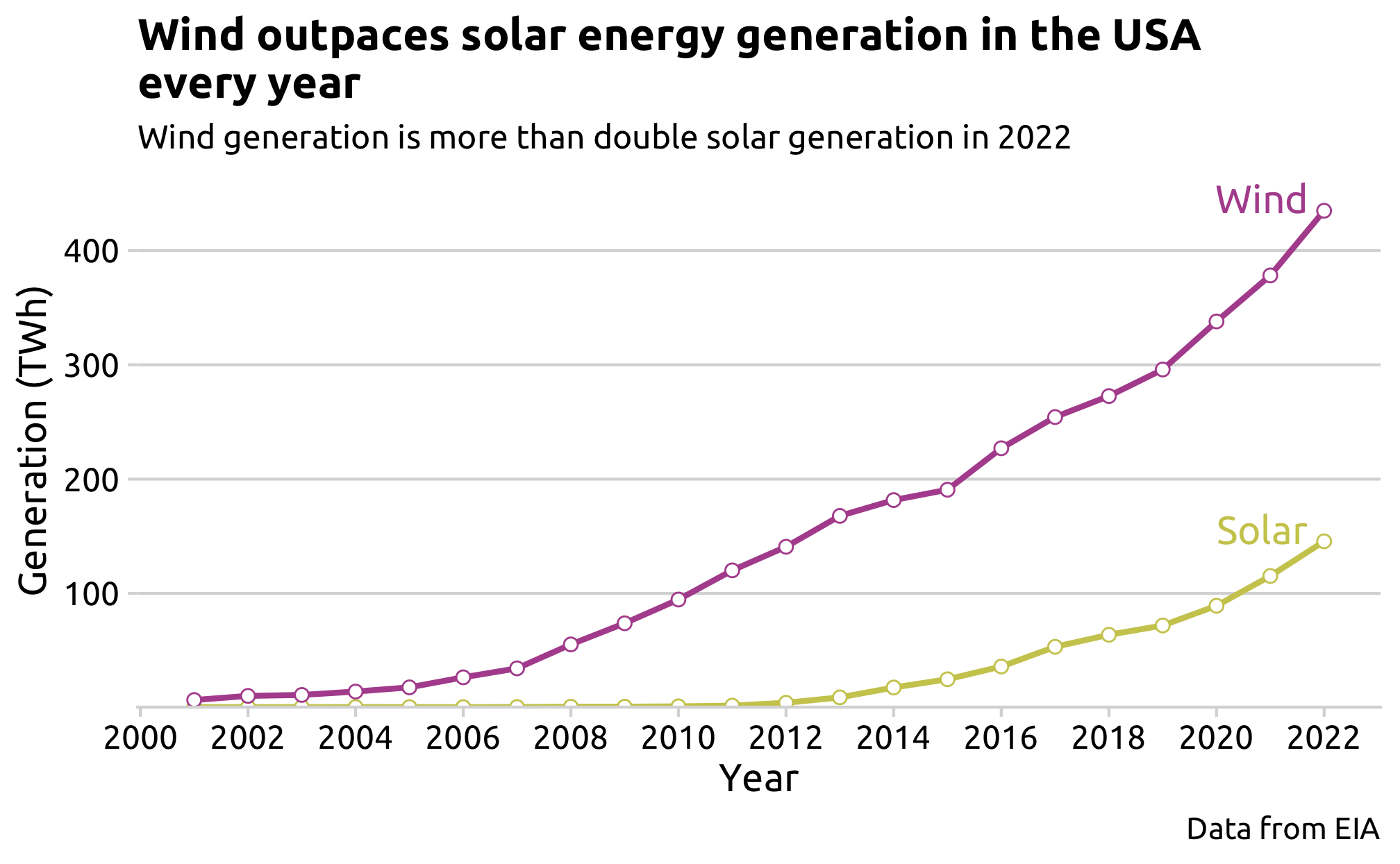
Using EIA data, the generation of solar and wind energy over time was explored.
Code
# 1. Solar generation data processingsolar_gen_path <-here('data', 'eia_solar_gen_raw.csv')solar_gen <-read_csv(solar_gen_path, skip =4) %>%clean_names() %>%select('month', 'united_states_thousand_megawatthours') %>%arrange(month) %>%mutate(month =dmy(paste('01', month)),month =format(month, '%Y-%m'),year =as.numeric(substr(month, 1, 4)) ) %>%filter(year <=2022) %>%group_by(year) %>%summarise(solar_gen_gwh =sum(united_states_thousand_megawatthours))write_csv(solar_gen, here('data', 'eia_solar_gen.csv'))# 2. Wind generation data processingwind_gen_path <-here('data', 'eia_wind_gen_raw.csv')wind_gen <-read_csv(wind_gen_path, skip =4) %>%clean_names() %>%select('month', 'united_states_thousand_megawatthours') %>%arrange(month) %>%mutate(month =dmy(paste('01', month)),month =format(month, '%Y-%m'),year =as.numeric(substr(month, 1, 4)) ) %>%filter(year <=2022) %>%group_by(year) %>%summarise(wind_gen_gwh =sum(united_states_thousand_megawatthours))write_csv(wind_gen, here('data', 'eia_wind_gen.csv'))# 3. Long format & exportingsolar_wind_gen_longer <-inner_join(solar_gen, wind_gen, by ='year') %>%pivot_longer(names_to ='energy_source',values_to ='gwh',cols =c('solar_gen_gwh', 'wind_gen_gwh'))write_csv(solar_wind_gen_longer,here('data', 'eia_solar_wind_gen_longer.csv'))# 4. Plot the Solar and Wind Generation over Timegeneration_plot <- solar_wind_gen_longer %>%ggplot(aes(x = year,y = gwh /1000,color = energy_source)) +geom_line(linewidth =1) +geom_point(fill ='white', size =2, shape =21) +geom_text(data =subset(solar_wind_gen_longer, year ==max(year)),aes(label =recode(energy_source, solar_gen_gwh ='Solar', wind_gen_gwh ='Wind')),nudge_x =-1.15,nudge_y =10,size =5,family ="Ubuntu") +labs(x ='Year',y ='Generation (TWh)',color ='Energy Source',title ='Wind outpaces solar energy generation in the USA\nevery year',subtitle ='Wind generation is more than double solar generation in 2022',caption ='Data from EIA') +scale_x_continuous(breaks =seq(2000, 2022, by =2)) +scale_y_continuous(expand =expand_scale(mult =c(0, 0.05))) +scale_color_manual(values =c('#ccca5d','#b2529d'))+theme_minimal_hgrid(font_family ='Ubuntu') +theme(legend.position ='none')ggsave(filename =here('figs_manu', '3_2_generation_plot.png'), plot = generation_plot,width =7,height =7/1.618)generation_plot
The generation of both solar and wind energy follows the expectations of being unimodal and widely spread. Both sources are increasing in annual generation and have yet to plateau, and the generation is widely-spread from about 0 to 150 and over 400 TWh for solar and wind, respectively. Solar generation did not start to grow until 2013, while wind generation has been increasing since 2001. Future exploration of the data can look into the deployment, size, and location of commercial solar and wind projects.
3.2 Cost of Solar and Wind Energy
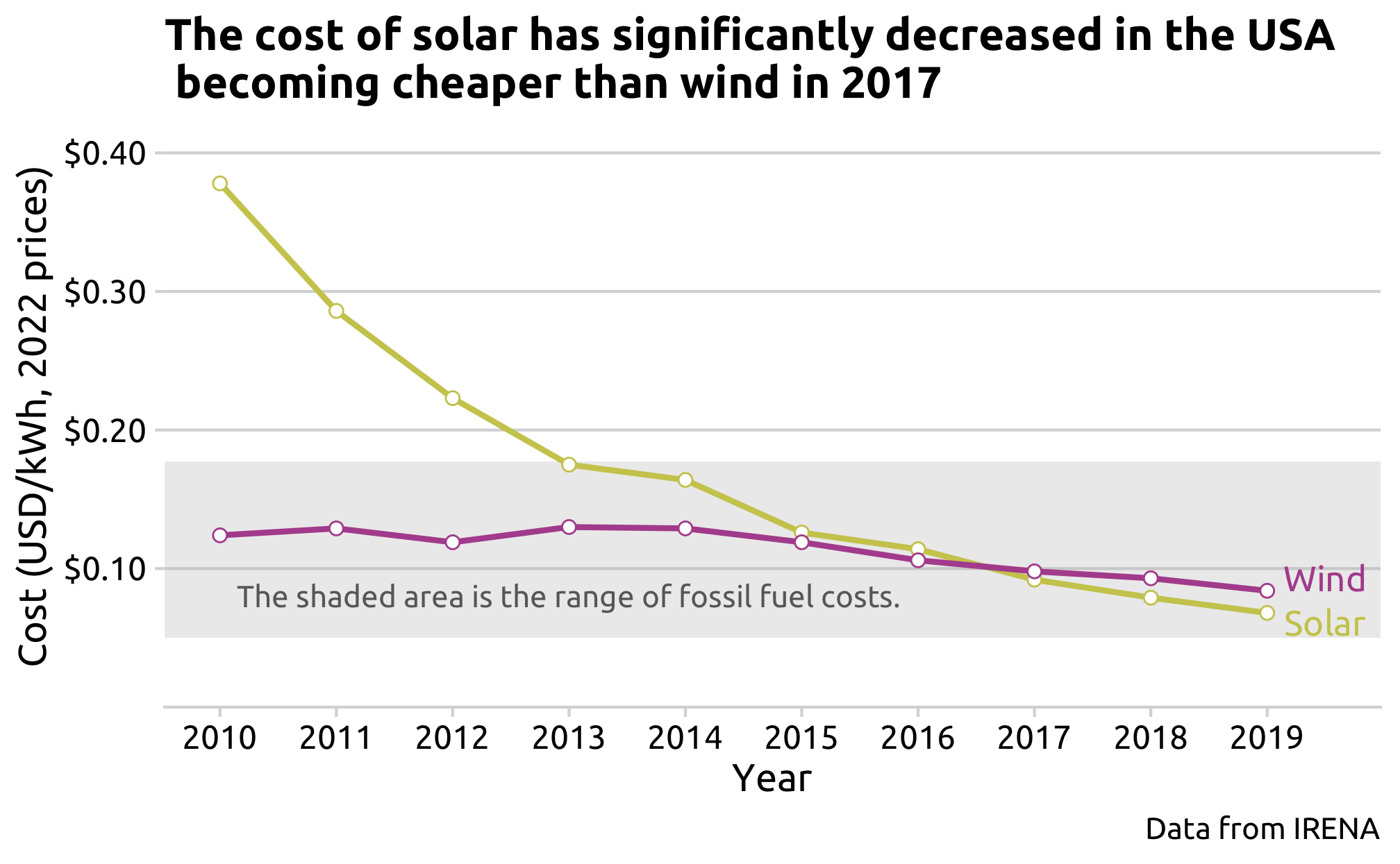
The cost of solar and wind was the first driver to be explored using data from IRENA.
Code
# 1. Read solar and wind cost data and merge to onesolar_cost <-read_csv(here('data', 'irena_solar_cost.csv'))wind_cost <-read_csv(here('data', 'irena_wind_cost.csv'))solar_wind_cost <-left_join(solar_cost, wind_cost, by ='year')# 2. Pivot to longer format and export to csvsolar_wind_cost_longer <- solar_wind_cost %>%pivot_longer(names_to ='energy_source',values_to ='cost',cols =-year)write_csv(solar_wind_cost_longer,here('data', 'irena_solar_wind_cost_longer.csv'))# 3. Create plot of solar and wind costs compared to fossil fuelscost_plot <- solar_wind_cost_longer %>%ggplot(aes(x = year,y = cost,color = energy_source)) +annotate('rect',xmin =-Inf, xmax =Inf,ymin =0.05, ymax =0.177,fill ='gray', alpha =0.3) +annotate('text',x =2013, y =0.08,color ='dimgray',label ='The shaded area is the range of fossil fuel costs.',family ="Ubuntu") +geom_line(linewidth =1) +geom_point(fill ='white', size =2, shape =21) +geom_text_repel(data =subset(solar_wind_cost_longer, year ==max(year)),aes(label =recode(energy_source, solar_cost_usd_per_kwh ='Solar', wind_cost_usd_per_kwh ='Wind')),nudge_x =0.5,nudge_y =0,size =4.5,family ="Ubuntu") +labs(x ='Year',y ='Cost (USD/kWh, 2022 prices)',color ='Energy Source',title ='The cost of solar has significantly decreased in the USA \n becoming cheaper than wind in 2017',caption ='Data from IRENA') +scale_x_continuous(breaks =seq(2010, 2019, by =1)) +scale_y_continuous(limits =c(0, 0.4), breaks =c(0.1, 0.2, 0.3, 0.4), expand =expand_scale(mult =c(0, 0.05)), labels = scales::dollar)+scale_color_manual(values =c('#ccca5d','#b2529d'))+theme_minimal_hgrid(font_family ='Ubuntu') +theme(legend.position ='none')ggsave(filename =here('figs_manu', '3_3_cost_plot.png'), plot = cost_plot,width =7,height =7/1.618)cost_plot
It was expected that the cost for renewables would be multimodal due to yearly variations and changes in administrations, but that the overall trend would be decreasing. In addition, the grouping was expected to range depending on the type of technology, specifically due to the capital cost elasticity. However, neither technology showed a multimodal distribution, rather the costs mainly remained relatively constant or decreased. The cost of solar energy generation shows a decreasing trend from around 0.38 to 0.07 USD/kWh and is more widely-spread than that of wind. Wind costs remained relatively constant around 0.13 to 0.08 USD/kWh. It makes sense that the cost of solar installation has a larger range than wind cost because of the technological solar panel advancements, which have made the capital cheaper, while wind turbines have not seen such progress. Furthermore, it is important to note that the cost of wind energy generation is the average value of on-shore and off-shore: it would be interesting to explore how wind costs vary depending on location within the USA.
The fossil fuel cost range is approximately 0.18 and 0.05 USD/kWh. For solar and wind to be economically competitive with fossil fuels, the costs needed to be similar if not less than that of fossil fuels. Interestingly, wind has been cost competitive with fossil fuels since 2010, but solar became competitive later in 2013.
When comparing the cost and generation trends, the cost competitiveness of solar energy with fossil fuels in 2013 coincides with the beginning of solar generation growth in 2013, which perhaps suggests that cost was the main factor behind solar’s delayed growth compared to wind. Since the cost of wind has remained relatively constant, cost does not seem to be the major contributor to wind’s growth. While solar did become cheaper than wind in 2017, wind continued to have a higher growth rate than solar in subsequent years.
3.3 Policies and Incentives
State policies was the second driver to be explored using data from DSIRE (Database of State Incentives for Renewables & Efficiency). Because the states receive federal funding for programs, like infrastructure, these state level policies likely coincide with federal level policies. Due to this state and federal relationship, congressional and presidential party alignment was explored as well (House), which usually coincides with more federal legislative activity.
Code
# 1. Scrape and save the raw policy data frame# 1.1 Read the html from local pathlaws_html_path <-here('data', 'dsire_laws_raw.html')laws_html <-read_html(laws_html_path)# 1.2 Scrape the table as a dflaws_table <- laws_html %>%html_nodes('table') %>% .[[1]] %>%html_table()# 1.3 Save the df to csvwrite_csv(laws_table, here('data', 'dsire_laws_raw.csv'))# 2. Construct solar and wind policy data frame# 2.1 Solar lawssolar_laws <-read_csv(here('data', 'dsire_laws_raw.csv')) %>%filter(grepl("Solar", Name, ignore.case =TRUE) |grepl("Solar", `Policy/Incentive Type`, ignore.case =TRUE)) %>%mutate(Created =as.integer(substr(Created, 7, 10))) %>%count(Created) %>%rename(year = Created, count_of_solar_laws = n)write_csv(solar_laws, here('data', 'dsire_solar_laws.csv'))# 2.2 Wind lawswind_laws <-read_csv(here('data', 'dsire_laws_raw.csv')) %>%filter(grepl("Wind", Name, ignore.case =TRUE) |grepl("Wind", `Policy/Incentive Type`, ignore.case =TRUE)) %>%mutate(Created =as.integer(substr(Created, 7, 10))) %>%count(Created) %>%rename(year = Created, count_of_wind_laws = n)write_csv(wind_laws, here('data', 'dsire_wind_laws.csv'))# 3. Plots of solar and wind laws# 3.1 Judge if congress is the same party as the presidentcongress_path <-here('data', 'congress.csv')congress <-read_csv(congress_path)# 3.2 Solar laws plotsolar_laws_plot <- solar_laws %>%left_join(congress, by ='year') %>%filter(year <=2020) %>%ggplot() +geom_col(aes(x = year, y = count_of_solar_laws, fill = both)) +geom_vline(xintercept =2000.5, color ='black', linetype ='solid') +geom_vline(xintercept =2008.5, color ='black', linetype ='solid') +geom_vline(xintercept =2016.5, color ='black', linetype ='solid') +annotate('text', x =2000.35, y =70, color ='#4c67a5', hjust =1,label ='Clinton', size =5, family ="Ubuntu") +annotate('text', x =2005, y =70, color ='#ad2730', hjust =1,label ='Bush', size =5, family ="Ubuntu") +annotate('text', x =2014, y =70, color ='#4c67a5', hjust =1,label ='Obama', size =5, family ="Ubuntu") +annotate('text', x =2019.75, y =70, color ='#ad2730', hjust =1,label ='Trump', size =5, family ="Ubuntu") +geom_label(data =data.frame(x =2004.5, y =50, label ='Both Congress and the \nPresident are of the \nsame political party'),aes(x = x, y = y, label = label),size =3.5, color ='#719847', family ="Ubuntu") +geom_curve(data =data.frame(x =2004.5, xend =2001.5, y =42, yend =10),mapping =aes(x = x, xend = xend, y = y, yend = yend),color ='#719847', size =0.5, curvature =0.1,arrow =arrow(length =unit(0.01, "npc"), type ="closed")) +geom_curve(data =data.frame(x =2004.5, xend =2005, y =42, yend =10),mapping =aes(x = x, xend = xend, y = y, yend = yend),color ='#719847', size =0.5, curvature =-0.1,arrow =arrow(length =unit(0.01, "npc"), type ="closed")) +geom_curve(data =data.frame(x =2004.5, xend =2009.5, y =42, yend =25),mapping =aes(x = x, xend = xend, y = y, yend = yend),color ='#719847', size =0.5, curvature =-0.1,arrow =arrow(length =unit(0.01, "npc"), type ="closed")) +scale_x_continuous(breaks =seq(2000, 2020, by =2),limits =c(1998, 2020),expand =expand_scale(mult =c(0, 0.05))) +scale_y_continuous(breaks =seq(0, 60, by =10),limits =c(0 , 70),expand =expand_scale(mult =c(0, 0.05))) +scale_fill_manual(values =c('#dbd9d6', '#719847')) +labs(x ='Year',y ='Number of Solar Policies',title ='State solar policies appear to coincide with\ndemocratic presidential terms',subtitle ='Alignment of political parties does not appear to impact legislation',caption ='Data from DSIRE') +theme_minimal_hgrid(font_family ='Ubuntu') +theme(legend.position ='none')ggsave(filename =here('figs_manu', '3_4_solar_laws_plot.png'), plot = solar_laws_plot,width =7,height =7/1.618)# 3.3 Wind policy plotwind_laws_plot <- wind_laws %>%left_join(congress, by ='year') %>%filter(year <=2020) %>%ggplot() +geom_col(aes(x = year, y = count_of_wind_laws, fill = both)) +geom_vline(xintercept =2000.5, color ='black', linetype ='solid') +geom_vline(xintercept =2008.5, color ='black', linetype ='solid') +geom_vline(xintercept =2016.5, color ='black', linetype ='solid') +annotate('text', x =2000.35, y =70, color ='#4c67a5', hjust =1,label ='Clinton', size =5, family ="Ubuntu") +annotate('text', x =2005, y =70, color ='#ad2730', hjust =1,label ='Bush', size =5, family ="Ubuntu") +annotate('text', x =2014, y =70, color ='#4c67a5', hjust =1,label ='Obama', size =5, family ="Ubuntu") +annotate('text', x =2019.75, y =70, color ='#ad2730', hjust =1,label ='Trump', size =5, family ="Ubuntu") +geom_label(data =data.frame(x =2004.5, y =50, label ='Both Congress and the \nPresident are of the \nsame political party'),aes(x = x, y = y, label = label),size =3.5, color ='#719847', family ="Ubuntu") +geom_curve(data =data.frame(x =2004.5, xend =2001.5, y =42, yend =10),mapping =aes(x = x, xend = xend, y = y, yend = yend),color ='#719847', size =0.5, curvature =0.1,arrow =arrow(length =unit(0.01, "npc"), type ="closed")) +geom_curve(data =data.frame(x =2004.5, xend =2005, y =42, yend =10),mapping =aes(x = x, xend = xend, y = y, yend = yend),color ='#719847', size =0.5, curvature =-0.1,arrow =arrow(length =unit(0.01, "npc"), type ="closed")) +geom_curve(data =data.frame(x =2004.5, xend =2009.5, y =42, yend =25),mapping =aes(x = x, xend = xend, y = y, yend = yend),color ='#719847', size =0.5, curvature =-0.1,arrow =arrow(length =unit(0.01, "npc"), type ="closed")) +scale_x_continuous(breaks =seq(2000, 2020, by =2),limits =c(1998, 2020),expand =expand_scale(mult =c(0, 0.05))) +scale_y_continuous(breaks =seq(0, 60, by =10),limits =c(0 , 70),expand =expand_scale(mult =c(0, 0.05))) +scale_fill_manual(values =c('#dbd9d6', '#719847')) +labs(x ='Year',y ='Number of Wind Policies',title ='State wind policies appear to coincide with\ndemocratic presidential terms',subtitle ='Alignment of political parties does not appear to impact legislation',caption ='Data from DSIRE') +theme_minimal_hgrid(font_family ='Ubuntu') +theme(legend.position ='none')ggsave(filename =here('figs_manu', '3_4_wind_laws_plot.png'), plot = wind_laws_plot,width =7,height =7/1.618)
It was expected that the number of policies would be multimodal and widely-spread due to changes in administration, both on a federal and state level. The plots for wind and solar policies support these expectations. The largest number of wind and solar policies occurred in 2000, which was near the end of Clinton’s presidential term, so more progressive policies may have been instituted at this time. There is a clear association of policies enacted depending on the presidential party: Clinton and Obama show higher policy counts than Trump and Bush, which makes sense since democrats are more progressive in renewable energy targets, producing a sort-of trickle down effect on the state-level polices. Interestingly, the enactment of these policies does not appear to be influenced by Congress and the president being of the same political party perhaps indicating non-partisan agreement for these policies: increasing solar and wind share of the state’s energy portfolio is not only an environmental benefit but can also provide more independence from the fossil fuel market, create new jobs, and opens the opportunity for the state to be a renewable energy technical leader. Finally, the figures have a high correlation due to both wind and solar being part of the larger renewable energy category and thus mentioned in the same bills, but generally solar policies outnumbered wind policies. Further research should explore how these state policies were distributed by state.
Relating these policies to generation, it makes sense that the largest number of wind and solar policies occurred in 2000 while the highest generation of wind and solar has been in the more recent years because there is usually a policy-implementation lag. Furthermore, the greater number of solar policies likely corresponds to the decreasing cost of solar through subsidies and credits, which corresponds to the more recent growth in solar.
3.4 Energy Research Budgets
The third and final driver to be explored was solar and wind RD&D budgets using data from the iea.
Code
# Store the wider format for later usesolar_wind_budget_wider <-read_csv(here('data', 'iea_solar_wind_budget_wider.csv') )# Generate the longer formatsolar_wind_budget_longer <-read_csv(here('data', 'iea_solar_wind_budget_wider.csv') ) %>%pivot_longer(cols =-year,names_to ='energy_source',values_to ='rdd_millions_usd')# Prepare the label data for the plotlabel_data <-subset(solar_wind_budget_longer, year ==max(year))label_data$nudge <-ifelse(label_data$energy_source =='solar_rdd_million_usd', 220, -100)# Sketch the plotbudget_plot <- solar_wind_budget_longer %>%ggplot(aes(x = year,y = rdd_millions_usd,color = energy_source)) +geom_line(linewidth =1) +geom_text(data = label_data,aes(label =recode(energy_source, solar_rdd_million_usd ='Solar', wind_rdd_million_usd ='Wind')),nudge_x =1.75,nudge_y = label_data$nudge, size =5,family ="Ubuntu") +labs(x ='Year',y ='RD&D Budget (Millions, 2022 USD)',color ='Energy Source',title ='Solar and wind energy RD&D budgets follow\nsimilar trends in the USA',subtitle ='Solar budget was higher than wind for all years',caption ='Data from IEA') +scale_x_continuous(limits =c(1970, 2018), breaks =seq(1975, 2015, by =5)) +theme_minimal_hgrid(font_family ='Ubuntu') +scale_color_manual(values =c('#ccca5d','#b2529d'))+scale_y_continuous(labels = scales::dollar)+theme(legend.position ='none') +# Carter boxgeom_label(data =data.frame(x =1972.6, y =990, label ='President Carter\nannounces\nNational Energy\nProgram'),aes(x = x, y = y, label = label),size =3.5, color ='#719847', color ='black',family ="Ubuntu") +annotate('point', x =1977 , y =578.5, color ='#719847', size =2) +annotate('point', x =1977 , y =83.0, color ='#719847', size =2) +geom_curve(data =data.frame(x =1973, xend =1977, y =790, yend =578.5),mapping =aes(x = x, xend = xend, y = y, yend = yend),color ='#719847', size =0.5, curvature =0.1,arrow =arrow(length =unit(0.01, "npc"),type ="closed")) +geom_curve(data =data.frame(x =1973, xend =1977, y =790, yend =83.0),mapping =aes(x = x, xend = xend, y = y, yend = yend),color ='#719847', size =0.5, curvature =0.1,arrow =arrow(length =unit(0.01, "npc"),type ="closed")) +# Treasury boxgeom_label(data =data.frame(x =2007, y =750, label ='Section 1603\nProgram begins'),aes(x = x, y = y, label = label),size =3.5, color ='#719847', color ='black',family ="Ubuntu") +annotate('point', x =2009 , y =531.5, color ='#719847', size =2) +annotate('point', x =2009 , y =247.7, color ='#719847', size =2) +geom_curve(data =data.frame(x =2007, xend =2009, y =650, yend =531.5),mapping =aes(x = x, xend = xend, y = y, yend = yend),color ='#719847', size =0.5, curvature =0.1,arrow =arrow(length =unit(0.01, "npc"),type ="closed")) +geom_curve(data =data.frame(x =2007, xend =2009, y =650, yend =247.7),mapping =aes(x = x, xend = xend, y = y, yend = yend),color ='#719847', size =0.5, curvature =0.1,arrow =arrow(length =unit(0.01, "npc"),type ="closed")) ggsave(filename =here('figs_manu', '3_5_budget_plot.png'), plot = budget_plot,width =7,height =7/1.618)budget_plot
It was expected that the amount of funding for renewable energy research would also be multimodal and widely-spread because of administration changes. The multimodal expectation was supported by the figure with peaks occurring around 1980, 1995, and 2010 for wind and solar, but solar was more wide-spread, while wind was more tightly-grouped. The boom in solar funding in the late 1970s could be related to the start of the environmental movement as well as President Carter’s announcement of the National Energy Program in 1977. The second major increase in funding around 2010 overlaps with Obama’s administration and the peak in state solar and wind policies (see previous figure). In addition, the research funding boom in 2010 may be due to the Section 1603 Program, which had to do with reimbursements for solar and wind installations, which drives efficiency research (1, 2).
Relating R&D back to generation, there appears to be a funding-implementation lag, as the most funding for solar occurred in the late 1970s and early 1980s, but the decline in solar costs and increase in solar generation is more recent. Although wind has less research funding than solar, it continues to generally have a higher growth rate in generation per year, which may indicate that research is not the primary driver of wind growth.
3.5 Correlations
To support the visual conclusions made between the drivers and generation, the correlation coefficients were calculated. All correlation calculations in this report have the method set as Spearman. The following relationships were expected:
The price of renewable energy is negatively correlated with renewable energy generation.
The number of promotional policies is positively correlated with renewable energy generation.
The amount of funding for renewable research is positively correlated with renewable energy generation.
3.5.1 Solar/Wind Generation vs 3 Drivers
Code
# 1. Merge and save solar and wind genmerged_solar_wind <- solar_cost %>%full_join(solar_gen, by ='year') %>%full_join(solar_laws, by ='year') %>%full_join(solar_wind_budget_wider, by ='year') %>%full_join(wind_cost, by ='year') %>%full_join(wind_gen, by ='year') %>%full_join(wind_laws, by ='year') %>%arrange(year)write_csv(merged_solar_wind, here('data', 'merged_solar_wind.csv'))# 2. Correlation coefficients between solar generation and other solar related variables:# cost (solar_cost_usd_per_kwh), laws (count_of_solar_laws), and budget(solar_rdd_million_usd)cor_solar_gen_solar_cost <-cor( merged_solar_wind$solar_gen_gwh, merged_solar_wind$solar_cost_usd_per_kwh,use ='pairwise.complete.obs',method ='spearman' )cor_solar_gen_solar_laws <-cor( merged_solar_wind$solar_gen_gwh, merged_solar_wind$count_of_solar_laws,use ='pairwise.complete.obs',method ='spearman' )cor_solar_gen_solar_rdd <-cor( merged_solar_wind$solar_gen_gwh, merged_solar_wind$solar_rdd_million_usd,use ='pairwise.complete.obs',method ='spearman' )# 3. Correlation coefficients for wind generation and other wind variablescor_wind_gen_wind_cost <-cor( merged_solar_wind$wind_gen_gwh, merged_solar_wind$wind_cost_usd_per_kwh,use ='pairwise.complete.obs',method ='spearman' )cor_wind_gen_wind_laws <-cor( merged_solar_wind$wind_gen_gwh, merged_solar_wind$count_of_wind_laws,use ='pairwise.complete.obs',method ='spearman' )cor_wind_gen_wind_rdd <-cor( merged_solar_wind$wind_gen_gwh, merged_solar_wind$wind_rdd_million_usd,use ='pairwise.complete.obs',method ='spearman' )# 4. Create dataframe of correlationscor_solar_wind <-data.frame(value_1 =c('Solar', 'Solar', 'Solar','Wind','Wind', 'Wind'),value_2 =c('Cost', 'Laws', 'Budgets','Cost', 'Laws', 'Budgets'),cor =c(cor_solar_gen_solar_cost, cor_solar_gen_solar_laws, cor_solar_gen_solar_rdd, cor_wind_gen_wind_cost, cor_wind_gen_wind_laws, cor_wind_gen_wind_rdd))write_csv(cor_solar_wind, here('data', 'cor_solar_wind.csv'))# 5. Summary table of the correlationscor_solar_wind %>%mutate(cor =round(cor, 2),cor =cell_spec( cor, 'html', color =ifelse( cor >0.5| cor <-0.5, 'white', 'black' ),background =ifelse( cor >0.5| cor <-0.5, 'cornflowerblue', 'white' ))) %>%kable(format ='html',escape =FALSE,align =c('l', 'l', 'l'),col.names =c('Energy Type', 'Compared Variable', 'Correlation'),caption ='Correlations of Solar/Wind Generation vs the Other 3 Variables') %>%kable_styling(bootstrap_options =c('striped', 'hover'))
Correlations of Solar/Wind Generation vs the Other 3 Variables
Energy Type
Compared Variable
Correlation
Solar
Cost
-1
Solar
Laws
-0.01
Solar
Budgets
0.46
Wind
Cost
-0.81
Wind
Laws
-0.08
Wind
Budgets
0.29
Support for two of the expected relationships was found: both solar and wind costs were negatively correlated with generation, and solar and wind budgets were positively correlated with generation. Solar and wind laws had an unexpected lack of correlation with generation, possibly indicating a policy-implementation lag.
3.5.2 Correlation Matrix
The main focus of this report was how these factors influenced solar and wind generation growth, but the relationships among these drivers are also an important consideration for synergy. The correlations among all variables were calculated and filtered for those greater than |0.8| indicating a high correlation.
Code
# 1. Merge and save datasets# 1.1 Solar datamerged_solar <- solar_cost %>%full_join(solar_gen, by ='year') %>%full_join(solar_laws, by ='year') %>%full_join(solar_wind_budget_wider %>%select(-wind_rdd_million_usd),by ='year') %>%arrange(year) %>%mutate(log_solar_cost =log(solar_cost_usd_per_kwh),log_solar_gen =log(solar_gen_gwh))write_csv(merged_solar, here('data', 'merged_solar.csv'))# 1.2 Wind datamerged_wind <- wind_cost %>%full_join(wind_gen, by ='year') %>%full_join(wind_laws, by ='year') %>%full_join(solar_wind_budget_wider %>%select(-solar_rdd_million_usd),by ='year') %>%arrange(year) %>%mutate(log_wind_cost =log(wind_cost_usd_per_kwh),log_wind_gen =log(wind_gen_gwh))write_csv(merged_wind, here('data', 'merged_wind.csv'))# 2. Correlation matrix for merged data# 2.1 Solar correlation matrixcor_matrix_solar <-cor( merged_solar[, sapply(merged_solar, is.numeric)],use ='pairwise.complete.obs',method ='spearman' ) %>%as.data.frame()# 2.2 Wind correlation matrixcor_matrix_wind <-cor( merged_wind[, sapply(merged_wind, is.numeric)],use ='pairwise.complete.obs',method ='spearman' ) %>%as.data.frame()# 3. Filter 'high' correlations with threshold of +/- 0.8# 3.1 High solar correlationscor_solar_high <- cor_matrix_solar %>%mutate(value_1 =row.names(.)) %>%gather(value_2, cor, -value_1) %>%filter(value_1 != value_2, cor >0.8| cor <-0.8) %>%mutate(min_var =pmin(value_1, value_2),max_var =pmax(value_1, value_2)) %>%distinct(min_var, max_var, .keep_all =TRUE) %>%select(-min_var, -max_var) %>%arrange(value_1) %>%filter((startsWith(value_1, "log") &startsWith(value_2, "log")) | (!startsWith(value_1, "log") &!startsWith(value_2, "log")))write_csv(cor_solar_high, here('data', 'cor_solar_high.csv'))# 3.2 High wind correlationscor_wind_high <- cor_matrix_wind %>%mutate(value_1 =row.names(.)) %>%gather(value_2, cor, -value_1) %>%filter(value_1 != value_2, cor >0.8| cor <-0.8) %>%mutate(min_var =pmin(value_1, value_2),max_var =pmax(value_1, value_2)) %>%distinct(min_var, max_var, .keep_all =TRUE) %>%select(-min_var, -max_var) %>%arrange(value_1) %>%filter((startsWith(value_1, "log") &startsWith(value_2, "log")) | (!startsWith(value_1, "log") &!startsWith(value_2, "log")))write_csv(cor_wind_high, here('data', 'cor_wind_high.csv'))# 4. Construct the 'high' correlation matrix table# There are 4 in solar and 3 in wind# Excluding time series, there are 2 in solar and 1 in windcor_matrix_high <-tibble(`No.`=seq(1,7),`Value 1`=c("Solar Cost", "Solar Gen", "log Solar Gen", "Solar RDD","Wind Cost", "Wind Gen", "log Wind Gen"),`Value 2`=c("Year", "Year", "log Solar Cost", "Solar Cost","Year", "Year", "log Wind Cost"),Correlation =c(round(cor_solar_high[2,3], 2),round(cor_solar_high[3,3], 2),round(cor_solar_high[1,3], 2),round(cor_solar_high[5,3], 2),round(cor_wind_high[2,3], 2),round(cor_wind_high[3,3], 2),round(cor_wind_high[1,3], 2)))cor_matrix_high_kable <- cor_matrix_high %>%kable(format ='html', escape =FALSE,align =c('c', 'l', 'l', 'c'),caption ='Correlations Matrix of High Correlations') %>%kable_styling(bootstrap_options =c('striped', 'hover'))cor_matrix_high_kable
Correlations Matrix of High Correlations
No.
Value 1
Value 2
Correlation
1
Solar Cost
Year
-1.00
2
Solar Gen
Year
0.98
3
log Solar Gen
log Solar Cost
-1.00
4
Solar RDD
Solar Cost
0.89
5
Wind Cost
Year
-0.81
6
Wind Gen
Year
1.00
7
log Wind Gen
log Wind Cost
-0.81
3.5.3 High Correlation Plots
Of the 7 high correlations, the team chose to skip over the time series correlations since they were previously depicted.
Code
# Plot 1: Log Solar Cost vs Log Solar Generationcor_plot_1 <- merged_solar_wind %>%filter(!is.na(solar_cost_usd_per_kwh) &!is.na(solar_gen_gwh)) %>%ggplot(aes(x =log(solar_cost_usd_per_kwh),y =log(solar_gen_gwh /1000))) +geom_point() +geom_smooth(method ='lm', se =FALSE, size =0.5,color ='cornflowerblue') +labs(x ='Solar Cost: log(USD/kWh)',y ='Solar Generation: log(TWh)',title='Log Solar Cost vs Log Solar Generation',subtitle ='Correlation = -1') +theme_minimal_grid(font_family ='Ubuntu')ggsave(filename =here('figs_manu', '3_6_cor_plot_1.png'), plot = cor_plot_1,width =6,height =6/1.618)# Plot 2: log Wind Cost vs log Wind Generationcor_plot_2 <- merged_solar_wind %>%filter(!is.na(wind_cost_usd_per_kwh) &!is.na(wind_gen_gwh)) %>%ggplot(aes(x =log(wind_cost_usd_per_kwh),y =log(wind_gen_gwh /1000))) +geom_point() +geom_smooth(method ='lm', se =FALSE, size =0.5,color ='cornflowerblue') +labs(x ='Wind Cost: log(USD/kWh)',y ='Wind Generation: log(TWh)',title='Log Wind Cost vs Log Wind Generation',subtitle ='Correlation = -0.81') +theme_minimal_grid(font_family ='Ubuntu')ggsave(filename =here('figs_manu', '3_6_cor_plot_2.png'), plot = cor_plot_2,width =6,height =6/1.618)# Plot 3: Solar RD&D vs Solar Costcor_plot_3 <- merged_solar_wind %>%filter(!is.na(solar_rdd_million_usd) &!is.na(solar_cost_usd_per_kwh)) %>%ggplot(aes(x = solar_rdd_million_usd,y = solar_cost_usd_per_kwh)) +geom_point() +geom_smooth(method ='lm', se =FALSE, size =0.5,color ='cornflowerblue') +labs(x ='Solar RD&D (USD)',y ='Solar Cost (USD / kWh)',title='Solar RD&D vs Solar Cost',subtitle ='Correlation = 0.89') +theme_minimal_grid(font_family ='Ubuntu')ggsave(filename =here('figs_manu', '3_6_cor_plot_3.png'), plot = cor_plot_3,width =6,height =6/1.618)
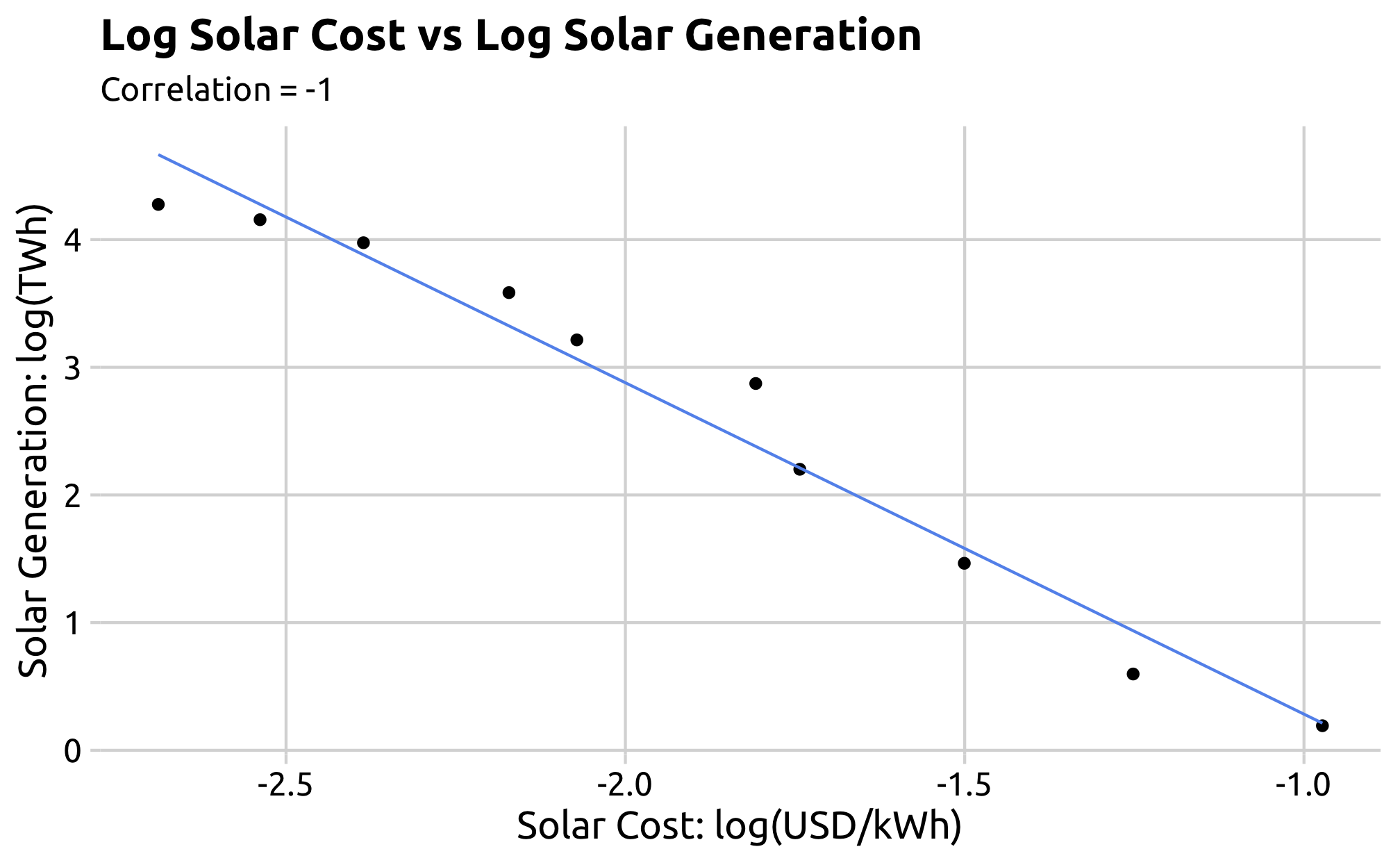
These correlation plots indicate the following findings:
The logarithm of cost and generation show a strong negative correlation, which is logical due to economies of scale: as solar and wind projects and thus generation increase, the price will fall. Also, as the capital cost get cheaper, there is a higher incentive to build these facilities.
Solar RD&D has strong positive correlation with solar costs: cheaper solar energy requires efficient construction of PV cells.
4. Conclusion
Overall, this study highlighted the complexity of understanding the growth of a new technology: technical advancements, economic incentives, and supporting policies need to be aligned. One key finding is that the decreasing cost of solar and wind energy is a contributor to their growth, but this relationship is stronger for solar than for wind highlighting solar’s rapid cost reduction that has spurred a more recent growth in generation. The wind and solar policies have almost no correlation with increased generation, thus the policy-implementation lag and variation in state implementation of solar and wind supportive policies may not be a direct driver for the growth, but rather a way to incentivize the economic and technical advancements that have a more direct impact on generation. Finally, the RD&D budget for solar and wind show a positive correlation with generation, but it is not strong perhaps indicating a funding-implementation lag as RD&D takes years to show a significant impact on technical efficiency and costs and eventually deployment.
Further analysis of these drivers is necessary to provide more significant conclusions about which drivers are more impactful for the United States’ growth in renewables. It is suggested that the USA continue a mix of economic, technical, and political drivers to see a continued growth in not only solar and wind but also other renewable energy sources. Suggested further analysis includes a focus on the distribution and strength of state government policies as well as the location and size of the solar and wind facilities across the US.
# 1. Calculate the summary and export to csvsummary_solar_gen <-summary(solar_gen$solar_gen_gwh)summary_solar_cost <-summary(solar_cost$solar_cost_usd_per_kwh)summary_solar_laws <-summary(solar_laws$count_of_solar_laws)summary_solar_budget <-summary(solar_wind_budget_wider$solar_rdd_million_usd)summary_solar_df <-data.frame(tier =names(summary_solar_gen),solar_gen_gwh =round(as.numeric(summary_solar_gen)),solar_cost_usd_per_kw =round(as.numeric(summary_solar_cost), 2),solar_laws_count =round(as.numeric(summary_solar_laws)),solar_budget_million_usd =round(as.numeric(summary_solar_budget)) )write_csv(summary_solar_df, here('data', 'summary_solar.csv'))# 2. Generate the table using kable()summary_solar_df %>%kable(format ='html',escape =FALSE,col.names =c('Tier','Electricity Generation (GWh)','Cost (USD/kWh)','Laws Count','RD&D Budget (Million USD)'),caption ='Summary of Solar') %>%kable_styling(bootstrap_options =c('striped', 'hover'))
Summary of Solar
Tier
Electricity Generation (GWh)
Cost (USD/kWh)
Laws Count
RD&D Budget (Million USD)
Min.
508
0.07
1
18
1st Qu.
584
0.10
4
133
Median
3072
0.15
9
173
Mean
29080
0.17
13
284
3rd Qu.
48979
0.21
21
277
Max.
145598
0.38
65
1168
Summary of Wind
Code
# 1. Calculate the summary and export to csvsummary_wind_gen <-summary(wind_gen$wind_gen_gwh)summary_wind_cost <-summary(wind_cost$wind_cost_usd_per_kwh)summary_wind_cost <- summary_wind_cost[!names(summary_wind_cost) =="NA's"]summary_wind_laws <-summary(wind_laws$count_of_wind_laws)summary_wind_budget <-summary(solar_wind_budget_wider$wind_rdd_million_usd)summary_wind_df <-data.frame(tier =names(summary_wind_gen),wind_gen_gwh =round(as.numeric(summary_wind_gen)),wind_cost_usd_per_kw =round(as.numeric(summary_wind_cost), 2),wind_laws_count =round(as.numeric(summary_wind_laws)),wind_budget_million_usd =round(as.numeric(summary_wind_budget)) )write_csv(summary_wind_df, here('data', 'summary_wind.csv'))# 2. Generate the table using kable()summary_wind_df %>%kable(format ='html',escape =FALSE,col.names =c('Tier','Electricity Generation (GWh)','Cost (USD/kWh)','Laws Count','RD&D Budget (Million USD)'),caption ='Summary of Wind') %>%kable_styling(bootstrap_options =c('striped', 'hover'))
Summary of Wind
Tier
Electricity Generation (GWh)
Cost (USD/kWh)
Laws Count
RD&D Budget (Million USD)
Min.
6737
0.08
1
0
1st Qu.
28554
0.10
2
32
Median
130499
0.12
8
57
Mean
152144
0.11
10
68
3rd Qu.
247475
0.13
10
83
Max.
434812
0.13
55
248
6.2 Dictionary of Correlations
This dictionary contains the correlation datasets.
Code
dict_cor <-data.frame(name =c('cor_matrix_high','cor_matrix_solar','cor_matrix_wind','cor_solar_wind','cor_solar_high','cor_wind_high'),type =c('A tibble: 7 × 4','A data frame: 6 × 6','A data frame: 6 × 6','A data frame: 8 × 3','A data frame: 5 × 3','A data frame: 2 × 3'),description =c('Correlation matrix of high correlation values','Correlation matrix of all solar related variables','Correlation matrix of all wind related variables','Correlation between generation and 3 other variables','Solar related correlations higher than 0.8','Wind related correlations higher than 0.8')) %>%mutate(count =row_number()) %>%select(count, everything())dict_cor %>%kable(format ='html',escape =FALSE,align =c('c', 'l', 'l', 'l'),col.names =c('No.', 'Name', 'Type', 'Description'),caption ='Dictionary of Correlations') %>%kable_styling(bootstrap_options =c('striped', 'hover'))
Dictionary of Correlations
No.
Name
Type
Description
1
cor_matrix_high
A tibble: 7 × 4
Correlation matrix of high correlation values
2
cor_matrix_solar
A data frame: 6 × 6
Correlation matrix of all solar related variables
3
cor_matrix_wind
A data frame: 6 × 6
Correlation matrix of all wind related variables
4
cor_solar_wind
A data frame: 8 × 3
Correlation between generation and 3 other variables
5
cor_solar_high
A data frame: 5 × 3
Solar related correlations higher than 0.8
6
cor_wind_high
A data frame: 2 × 3
Wind related correlations higher than 0.8
6.3 Dictionary of Files
This is a complete dictionary of files. The files can be accessed in the “data” folder. In the dictionary, there are 4 columns:
Name - The name of the file.
Type - The type of the file. In our case, we have CSV, HTML, and Excel.
Source - The source of the file. “Generated” means it is generated by R codes; “Raw” means Its either directly downloaded or scrapped from the website.
Description - A brief description of the file.
The dictionary is in alphabetical order.
Code
dict_file <-data.frame(name =c('congress','cor_solar_wind','dsire_laws_raw','dsire_solar_laws','dsire_wind_laws','eia_solar_gen_raw','eia_solar_gen','eia_solar_wind_gen_longer','eia_wind_gen_raw','eia_wind_gen','cor_solar_high','cor_wind_high','iea_solar_wind_budget_wider','irena_solar_cost','irena_solar_wind_cost_longer','irena_solar_wind_international_long','irena_solar_wind_international_raw','irena_wind_cost','merged_solar_wind','merged_solar','merged_wind','summary_solar','summary_wind','dsire_laws_raw','irena_costs_raw'),type =c('CSV', 'CSV', 'CSV', 'CSV', 'CSV','CSV', 'CSV', 'CSV', 'CSV', 'CSV','CSV', 'CSV', 'CSV', 'CSV', 'CSV','CSV', 'CSV', 'CSV', 'CSV', 'CSV','CSV', 'CSV', 'CSV', 'HTML', 'Excel'),source =c('Raw', 'Generated', 'Raw', 'Generated','Generated','Raw', 'Generated', 'Generated','Raw', 'Generated', 'Generated', 'Generated','Raw', 'Generated', 'Generated', 'Generated', 'Raw','Generated', 'Generated', 'Generated', 'Generated','Generated', 'Generated', 'Raw', 'Raw'),description =c('Parties of congress and present','Correlation between generation and 3 other variables','Laws and incentives count from DSIRE','Solar laws and incentives count','Wind laws and incentives count','Monthly solar electricity generation from EIA','Annual solar electricity generation','Longer version of annual solar/wind generation','Monthly wind electricity generation from EIA','Annual wind electricity generation','Solar related correlations higher than 0.8','Wind related correlations higher than 0.8','Wider version of solar/wind RD&D budgets from IEA','Annual average solar cost','Longer version of solar/wind generation cost','Longer version of international solar/wind gen','Wider version of international solad/wind gen','Annual average wind cost','Merged dataset of both solar, wind','Merged dataset of solar','Merged dataset of wind','Summary dataset of solar','Summary dataset of wind','Scraped law count data from DSIRE','Renewable power generation cost data from IRENA')) %>%mutate(count =row_number()) %>%select(count, everything())dict_file %>%kable(format ='html',escape =FALSE,align =c('c', 'l', 'l', 'l', 'l'),col.names =c('No.', 'Name', 'Type', 'Source', 'Description'),caption ='Dictionary of Data Files') %>%kable_styling(bootstrap_options =c('striped', 'hover'))
Dictionary of Data Files
No.
Name
Type
Source
Description
1
congress
CSV
Raw
Parties of congress and present
2
cor_solar_wind
CSV
Generated
Correlation between generation and 3 other variables
3
dsire_laws_raw
CSV
Raw
Laws and incentives count from DSIRE
4
dsire_solar_laws
CSV
Generated
Solar laws and incentives count
5
dsire_wind_laws
CSV
Generated
Wind laws and incentives count
6
eia_solar_gen_raw
CSV
Raw
Monthly solar electricity generation from EIA
7
eia_solar_gen
CSV
Generated
Annual solar electricity generation
8
eia_solar_wind_gen_longer
CSV
Generated
Longer version of annual solar/wind generation
9
eia_wind_gen_raw
CSV
Raw
Monthly wind electricity generation from EIA
10
eia_wind_gen
CSV
Generated
Annual wind electricity generation
11
cor_solar_high
CSV
Generated
Solar related correlations higher than 0.8
12
cor_wind_high
CSV
Generated
Wind related correlations higher than 0.8
13
iea_solar_wind_budget_wider
CSV
Raw
Wider version of solar/wind RD&D budgets from IEA
14
irena_solar_cost
CSV
Generated
Annual average solar cost
15
irena_solar_wind_cost_longer
CSV
Generated
Longer version of solar/wind generation cost
16
irena_solar_wind_international_long
CSV
Generated
Longer version of international solar/wind gen
17
irena_solar_wind_international_raw
CSV
Raw
Wider version of international solad/wind gen
18
irena_wind_cost
CSV
Generated
Annual average wind cost
19
merged_solar_wind
CSV
Generated
Merged dataset of both solar, wind
20
merged_solar
CSV
Generated
Merged dataset of solar
21
merged_wind
CSV
Generated
Merged dataset of wind
22
summary_solar
CSV
Generated
Summary dataset of solar
23
summary_wind
CSV
Generated
Summary dataset of wind
24
dsire_laws_raw
HTML
Raw
Scraped law count data from DSIRE
25
irena_costs_raw
Excel
Raw
Renewable power generation cost data from IRENA
6.4 Dictionary of Solar and Wind Datasets
This is a dictionary of solar and wind related datasets that are generated in this report. The majority of the datasets overlap with the file dictionary, and they have same or similar names.
Code
dict_solar_wind <-data.frame(name =c('merged_solar','merged_solar_wind','merged_wind','solar_cost','solar_gen','solar_international','solar_laws','solar_wind_budget_longer','solar_wind_budget_wider','solar_wind_cost','solar_wind_cost_longer','solar_wind_gen_longer','sum_international','summary_solar_df','summary_wind_df','top_5_solar','top_5_wind','us_elec_gen','wind_cost','wind_gen','wind_international','wind_laws'),type =c('A tibble: 50 × 7','A tibble: 50 × 10','A tibble: 49 × 6','A tibble: 10 × 2','A tibble: 22 × 2','A tibble: 5,302 x 4','A tibble: 20 × 2','A tibble: 84 × 3','A tibble: 42 × 3','A tibble: 10 × 3','A tibble: 20 × 3','A tibble: 44 × 3','A tibble: 482 x 3','A data frame: 6 x 5','A data frame: 6 x 5','A tibble: 5 × 4','A tibble: 5 × 4','A tibble: 4 × 2','A tibble: 36 × 2','A tibble: 22 × 2','A tibble: 5,302 × 4','A tibble: 17 × 2'),description =c('Merged dataset of solar data','Merged dataset of all solar and wind data','Merged dataset of wind data','Annual average solar cost','Annual solar electricity generation','International solar generation by country','Solar laws and incentives count','Longer version of solar/wind RD&D budgets','Wider version of solar/wind RD&D budgets','Solar/wind cost','Longer version of solar/wind cost','Longer version of annual solar/wind generation','Sum of international solar gen by country','Summary dataset of solar','Summary dataset of wind','Solar gen of top 5 countries in 2021','Wind gen of top 5 countries in 2021','Percentage of energy source in US in 2022','Annual average wind cost','Annual wind electricity generation','International wind generation by country','Wind laws and incentives count')) %>%mutate(count =row_number()) %>%select(count, everything())dict_solar_wind %>%kable(format ='html',escape =FALSE,align =c('c', 'l', 'l', 'l'),col.names =c('No.', 'Name', 'Type', 'Description'),caption ='Dictionary of Solar and Wind Datasets') %>%kable_styling(bootstrap_options =c('striped', 'hover'))
Dictionary of Solar and Wind Datasets
No.
Name
Type
Description
1
merged_solar
A tibble: 50 × 7
Merged dataset of solar data
2
merged_solar_wind
A tibble: 50 × 10
Merged dataset of all solar and wind data
3
merged_wind
A tibble: 49 × 6
Merged dataset of wind data
4
solar_cost
A tibble: 10 × 2
Annual average solar cost
5
solar_gen
A tibble: 22 × 2
Annual solar electricity generation
6
solar_international
A tibble: 5,302 x 4
International solar generation by country
7
solar_laws
A tibble: 20 × 2
Solar laws and incentives count
8
solar_wind_budget_longer
A tibble: 84 × 3
Longer version of solar/wind RD&D budgets
9
solar_wind_budget_wider
A tibble: 42 × 3
Wider version of solar/wind RD&D budgets
10
solar_wind_cost
A tibble: 10 × 3
Solar/wind cost
11
solar_wind_cost_longer
A tibble: 20 × 3
Longer version of solar/wind cost
12
solar_wind_gen_longer
A tibble: 44 × 3
Longer version of annual solar/wind generation
13
sum_international
A tibble: 482 x 3
Sum of international solar gen by country
14
summary_solar_df
A data frame: 6 x 5
Summary dataset of solar
15
summary_wind_df
A data frame: 6 x 5
Summary dataset of wind
16
top_5_solar
A tibble: 5 × 4
Solar gen of top 5 countries in 2021
17
top_5_wind
A tibble: 5 × 4
Wind gen of top 5 countries in 2021
18
us_elec_gen
A tibble: 4 × 2
Percentage of energy source in US in 2022
19
wind_cost
A tibble: 36 × 2
Annual average wind cost
20
wind_gen
A tibble: 22 × 2
Annual wind electricity generation
21
wind_international
A tibble: 5,302 × 4
International wind generation by country
22
wind_laws
A tibble: 17 × 2
Wind laws and incentives count
6.5 Miscellaneous
There are also other datasets that are not included in the above dictionaries:
There are 3 plots named as cor_plot_1 through cor_plot_3. These are the correlation plots shown in [3.6.3 High Correlation Plots]. The other plots are shown directly and are not stored as variables or datasets.
There are also some other datasets like label_data, laws_html, laws_table, etc. They are used to temporarily store values.
6.6 All Code
Code
knitr::opts_chunk$set(comment ="#>",fig.align ="center",fig.show ="hold",fig.width =7,fig.asp =0.618,fig.retina =3,fig.path ="figs_auto/",out.width ="90%")library(tidyverse)library(here)library(janitor)library(lubridate)library(rvest)library(gridExtra)library(kableExtra)library(cowplot)library(ggrepel)library(gganimate)library(plotly)library(reactable)us_elec_gen <-tibble(Type =c("Renewables", "Natural Gas", "Nuclear", "Coal"),Percentage =c(0.23, 0.39, 0.18, 0.19))us_elec_bar <- us_elec_gen %>%ggplot(aes(x =reorder(Type, -Percentage),y = Percentage,fill = Type)) +geom_col(width =0.5) +scale_fill_manual(values =c("Renewables"="#719847","Natural Gas"="gray","Nuclear"="gray","Coal"="dimgray")) +geom_text(aes(label = scales::percent(Percentage)), vjust =-0.3,size =5,family ="Ubuntu") +scale_y_continuous(expand =expansion(mult =c(0, 0.15)),labels = scales::percent_format()) +theme_minimal_hgrid(font_family ="Ubuntu") +theme(legend.position ="none",axis.text.x =element_text(size =11)) +labs(x ="Energy Type",y ="Electricity Share",title ="Renewables outnumber coal for electricity\ngeneration in 2022",caption ="Data from BCSE")us_elec_bar# 1. Load and clean data of international solar and wind gendrop <-c('World', 'Asia', 'Europe', 'North America','European Union', 'South America', 'Eurasia', 'Africa')internationalPath <-here('data', 'irena_solar_wind_international_raw.csv')international <-read_csv(internationalPath, skip =2) %>%rename(Country ='Region/country/area') %>%pivot_longer(names_to ='Year',values_to ='Generation',cols ='2000':'2021') %>%mutate(Year =as.numeric(Year) ) %>%filter(!Country %in% drop)international %>%write_csv(here('data', 'irena_solar_wind_international_long.csv'))# 2. International Solar Generation# 2.1 Solar gen data framesolar_international <- international %>%filter(Technology =='Solar')# 2.2 Top 5 solar producers in 2021top_5_solar <- solar_international %>%filter(Year =='2021') %>%arrange(desc(Generation)) %>%slice(1:5)# 2.3 Plot of top 5 solar producerssolar_international_plot <-ggplot(solar_international %>%filter(Country %in%c(top_5_solar$Country)),aes(x = Year, y = Generation/1000, group = Country, color = Country)) +geom_line(linewidth =1) +geom_text_repel(data = top_5_solar,aes(label = Country),hjust =0, nudge_x =1, direction ="y",size =5, segment.color =NA,family ="Ubuntu") +scale_x_continuous(breaks =seq(2000, 2021, 3),expand =expansion(add =c(1, 5))) +scale_y_continuous(expand =expand_scale(mult =c(0, 0.05))) +labs(x ='Year',y ='Generation (TWh)',title ='United States is the second highest producer of\nsolar energy',subtitle ='Top 5 producers of solar energy in 2021',caption ='Data from IRENA') +scale_color_manual(values =c('#719847','#ccca5d','#b2529d','#4c67a5','#a5734c')) +theme_minimal_hgrid(font_family ='Ubuntu') +theme(legend.position ='none')ggsave(filename =here('figs_manu', '3_1_solar_inter_plot.png'), plot = solar_international_plot,width =8,height =8/1.618)# 3. International Wind Generation# 3.1 Wind gen data framewind_international <- international %>%filter(Technology =='Wind')# 3.2 Top 5 wind producers in 2021top_5_wind <- wind_international %>%filter(Year =='2021') %>%arrange(desc(Generation)) %>%slice(1:5)# 3.3 Plot of top 5 wind producerswind_international_plot <-ggplot(wind_international %>%filter(Country %in%c(top_5_wind$Country)),aes(x = Year, y = Generation/1000, group = Country, color = Country)) +geom_line(linewidth =1) +geom_text_repel(data = top_5_wind,aes(label = Country),hjust =0, nudge_x =1, direction ="y",size =5, segment.color =NA,family ="Ubuntu") +scale_x_continuous(breaks =seq(2000, 2021, 3),expand =expansion(add =c(1, 5))) +scale_y_continuous(expand =expand_scale(mult =c(0, 0.05))) +labs(x ='Year',y ='Generation (TWh)',title ='United States is the second highest producer of\nwind energy',subtitle ='Top 5 producers of wind energy in 2021',caption ='Data from IRENA') +scale_color_manual(values =c('#719847','#ccca5d','#b2529d','#4c67a5','#a5734c')) +theme_minimal_hgrid(font_family ='Ubuntu') +theme(legend.position ='none')ggsave(filename =here('figs_manu', '3_1_wind_inter_plot.png'), plot = wind_international_plot,width =8,height =8/1.618)# 4. International summary tablesum_international <- international %>%group_by(Country, Technology) %>%summarize(`Total Generation (tWh)`=sum(Generation, na.rm =TRUE)) %>%rename(`Technology (Solar or Wind)`= Technology)sum_international_table <- sum_international %>%reactable(searchable =TRUE,highlight =TRUE,filterable =TRUE,defaultPageSize =5,showPageSizeOptions =TRUE,pageSizeOptions =c(5, 10, 15) )solar_international_plotwind_international_plotsum_international_table# 1. Solar generation data processingsolar_gen_path <-here('data', 'eia_solar_gen_raw.csv')solar_gen <-read_csv(solar_gen_path, skip =4) %>%clean_names() %>%select('month', 'united_states_thousand_megawatthours') %>%arrange(month) %>%mutate(month =dmy(paste('01', month)),month =format(month, '%Y-%m'),year =as.numeric(substr(month, 1, 4)) ) %>%filter(year <=2022) %>%group_by(year) %>%summarise(solar_gen_gwh =sum(united_states_thousand_megawatthours))write_csv(solar_gen, here('data', 'eia_solar_gen.csv'))# 2. Wind generation data processingwind_gen_path <-here('data', 'eia_wind_gen_raw.csv')wind_gen <-read_csv(wind_gen_path, skip =4) %>%clean_names() %>%select('month', 'united_states_thousand_megawatthours') %>%arrange(month) %>%mutate(month =dmy(paste('01', month)),month =format(month, '%Y-%m'),year =as.numeric(substr(month, 1, 4)) ) %>%filter(year <=2022) %>%group_by(year) %>%summarise(wind_gen_gwh =sum(united_states_thousand_megawatthours))write_csv(wind_gen, here('data', 'eia_wind_gen.csv'))# 3. Long format & exportingsolar_wind_gen_longer <-inner_join(solar_gen, wind_gen, by ='year') %>%pivot_longer(names_to ='energy_source',values_to ='gwh',cols =c('solar_gen_gwh', 'wind_gen_gwh'))write_csv(solar_wind_gen_longer,here('data', 'eia_solar_wind_gen_longer.csv'))# 4. Plot the Solar and Wind Generation over Timegeneration_plot <- solar_wind_gen_longer %>%ggplot(aes(x = year,y = gwh /1000,color = energy_source)) +geom_line(linewidth =1) +geom_point(fill ='white', size =2, shape =21) +geom_text(data =subset(solar_wind_gen_longer, year ==max(year)),aes(label =recode(energy_source, solar_gen_gwh ='Solar', wind_gen_gwh ='Wind')),nudge_x =-1.15,nudge_y =10,size =5,family ="Ubuntu") +labs(x ='Year',y ='Generation (TWh)',color ='Energy Source',title ='Wind outpaces solar energy generation in the USA\nevery year',subtitle ='Wind generation is more than double solar generation in 2022',caption ='Data from EIA') +scale_x_continuous(breaks =seq(2000, 2022, by =2)) +scale_y_continuous(expand =expand_scale(mult =c(0, 0.05))) +scale_color_manual(values =c('#ccca5d','#b2529d'))+theme_minimal_hgrid(font_family ='Ubuntu') +theme(legend.position ='none')ggsave(filename =here('figs_manu', '3_2_generation_plot.png'), plot = generation_plot,width =7,height =7/1.618)generation_plot# 1. Read solar and wind cost data and merge to onesolar_cost <-read_csv(here('data', 'irena_solar_cost.csv'))wind_cost <-read_csv(here('data', 'irena_wind_cost.csv'))solar_wind_cost <-left_join(solar_cost, wind_cost, by ='year')# 2. Pivot to longer format and export to csvsolar_wind_cost_longer <- solar_wind_cost %>%pivot_longer(names_to ='energy_source',values_to ='cost',cols =-year)write_csv(solar_wind_cost_longer,here('data', 'irena_solar_wind_cost_longer.csv'))# 3. Create plot of solar and wind costs compared to fossil fuelscost_plot <- solar_wind_cost_longer %>%ggplot(aes(x = year,y = cost,color = energy_source)) +annotate('rect',xmin =-Inf, xmax =Inf,ymin =0.05, ymax =0.177,fill ='gray', alpha =0.3) +annotate('text',x =2013, y =0.08,color ='dimgray',label ='The shaded area is the range of fossil fuel costs.',family ="Ubuntu") +geom_line(linewidth =1) +geom_point(fill ='white', size =2, shape =21) +geom_text_repel(data =subset(solar_wind_cost_longer, year ==max(year)),aes(label =recode(energy_source, solar_cost_usd_per_kwh ='Solar', wind_cost_usd_per_kwh ='Wind')),nudge_x =0.5,nudge_y =0,size =4.5,family ="Ubuntu") +labs(x ='Year',y ='Cost (USD/kWh, 2022 prices)',color ='Energy Source',title ='The cost of solar has significantly decreased in the USA \n becoming cheaper than wind in 2017',caption ='Data from IRENA') +scale_x_continuous(breaks =seq(2010, 2019, by =1)) +scale_y_continuous(limits =c(0, 0.4), breaks =c(0.1, 0.2, 0.3, 0.4), expand =expand_scale(mult =c(0, 0.05)), labels = scales::dollar)+scale_color_manual(values =c('#ccca5d','#b2529d'))+theme_minimal_hgrid(font_family ='Ubuntu') +theme(legend.position ='none')ggsave(filename =here('figs_manu', '3_3_cost_plot.png'), plot = cost_plot,width =7,height =7/1.618)cost_plot# 1. Scrape and save the raw policy data frame# 1.1 Read the html from local pathlaws_html_path <-here('data', 'dsire_laws_raw.html')laws_html <-read_html(laws_html_path)# 1.2 Scrape the table as a dflaws_table <- laws_html %>%html_nodes('table') %>% .[[1]] %>%html_table()# 1.3 Save the df to csvwrite_csv(laws_table, here('data', 'dsire_laws_raw.csv'))# 2. Construct solar and wind policy data frame# 2.1 Solar lawssolar_laws <-read_csv(here('data', 'dsire_laws_raw.csv')) %>%filter(grepl("Solar", Name, ignore.case =TRUE) |grepl("Solar", `Policy/Incentive Type`, ignore.case =TRUE)) %>%mutate(Created =as.integer(substr(Created, 7, 10))) %>%count(Created) %>%rename(year = Created, count_of_solar_laws = n)write_csv(solar_laws, here('data', 'dsire_solar_laws.csv'))# 2.2 Wind lawswind_laws <-read_csv(here('data', 'dsire_laws_raw.csv')) %>%filter(grepl("Wind", Name, ignore.case =TRUE) |grepl("Wind", `Policy/Incentive Type`, ignore.case =TRUE)) %>%mutate(Created =as.integer(substr(Created, 7, 10))) %>%count(Created) %>%rename(year = Created, count_of_wind_laws = n)write_csv(wind_laws, here('data', 'dsire_wind_laws.csv'))# 3. Plots of solar and wind laws# 3.1 Judge if congress is the same party as the presidentcongress_path <-here('data', 'congress.csv')congress <-read_csv(congress_path)# 3.2 Solar laws plotsolar_laws_plot <- solar_laws %>%left_join(congress, by ='year') %>%filter(year <=2020) %>%ggplot() +geom_col(aes(x = year, y = count_of_solar_laws, fill = both)) +geom_vline(xintercept =2000.5, color ='black', linetype ='solid') +geom_vline(xintercept =2008.5, color ='black', linetype ='solid') +geom_vline(xintercept =2016.5, color ='black', linetype ='solid') +annotate('text', x =2000.35, y =70, color ='#4c67a5', hjust =1,label ='Clinton', size =5, family ="Ubuntu") +annotate('text', x =2005, y =70, color ='#ad2730', hjust =1,label ='Bush', size =5, family ="Ubuntu") +annotate('text', x =2014, y =70, color ='#4c67a5', hjust =1,label ='Obama', size =5, family ="Ubuntu") +annotate('text', x =2019.75, y =70, color ='#ad2730', hjust =1,label ='Trump', size =5, family ="Ubuntu") +geom_label(data =data.frame(x =2004.5, y =50, label ='Both Congress and the \nPresident are of the \nsame political party'),aes(x = x, y = y, label = label),size =3.5, color ='#719847', family ="Ubuntu") +geom_curve(data =data.frame(x =2004.5, xend =2001.5, y =42, yend =10),mapping =aes(x = x, xend = xend, y = y, yend = yend),color ='#719847', size =0.5, curvature =0.1,arrow =arrow(length =unit(0.01, "npc"), type ="closed")) +geom_curve(data =data.frame(x =2004.5, xend =2005, y =42, yend =10),mapping =aes(x = x, xend = xend, y = y, yend = yend),color ='#719847', size =0.5, curvature =-0.1,arrow =arrow(length =unit(0.01, "npc"), type ="closed")) +geom_curve(data =data.frame(x =2004.5, xend =2009.5, y =42, yend =25),mapping =aes(x = x, xend = xend, y = y, yend = yend),color ='#719847', size =0.5, curvature =-0.1,arrow =arrow(length =unit(0.01, "npc"), type ="closed")) +scale_x_continuous(breaks =seq(2000, 2020, by =2),limits =c(1998, 2020),expand =expand_scale(mult =c(0, 0.05))) +scale_y_continuous(breaks =seq(0, 60, by =10),limits =c(0 , 70),expand =expand_scale(mult =c(0, 0.05))) +scale_fill_manual(values =c('#dbd9d6', '#719847')) +labs(x ='Year',y ='Number of Solar Policies',title ='State solar policies appear to coincide with\ndemocratic presidential terms',subtitle ='Alignment of political parties does not appear to impact legislation',caption ='Data from DSIRE') +theme_minimal_hgrid(font_family ='Ubuntu') +theme(legend.position ='none')ggsave(filename =here('figs_manu', '3_4_solar_laws_plot.png'), plot = solar_laws_plot,width =7,height =7/1.618)# 3.3 Wind policy plotwind_laws_plot <- wind_laws %>%left_join(congress, by ='year') %>%filter(year <=2020) %>%ggplot() +geom_col(aes(x = year, y = count_of_wind_laws, fill = both)) +geom_vline(xintercept =2000.5, color ='black', linetype ='solid') +geom_vline(xintercept =2008.5, color ='black', linetype ='solid') +geom_vline(xintercept =2016.5, color ='black', linetype ='solid') +annotate('text', x =2000.35, y =70, color ='#4c67a5', hjust =1,label ='Clinton', size =5, family ="Ubuntu") +annotate('text', x =2005, y =70, color ='#ad2730', hjust =1,label ='Bush', size =5, family ="Ubuntu") +annotate('text', x =2014, y =70, color ='#4c67a5', hjust =1,label ='Obama', size =5, family ="Ubuntu") +annotate('text', x =2019.75, y =70, color ='#ad2730', hjust =1,label ='Trump', size =5, family ="Ubuntu") +geom_label(data =data.frame(x =2004.5, y =50, label ='Both Congress and the \nPresident are of the \nsame political party'),aes(x = x, y = y, label = label),size =3.5, color ='#719847', family ="Ubuntu") +geom_curve(data =data.frame(x =2004.5, xend =2001.5, y =42, yend =10),mapping =aes(x = x, xend = xend, y = y, yend = yend),color ='#719847', size =0.5, curvature =0.1,arrow =arrow(length =unit(0.01, "npc"), type ="closed")) +geom_curve(data =data.frame(x =2004.5, xend =2005, y =42, yend =10),mapping =aes(x = x, xend = xend, y = y, yend = yend),color ='#719847', size =0.5, curvature =-0.1,arrow =arrow(length =unit(0.01, "npc"), type ="closed")) +geom_curve(data =data.frame(x =2004.5, xend =2009.5, y =42, yend =25),mapping =aes(x = x, xend = xend, y = y, yend = yend),color ='#719847', size =0.5, curvature =-0.1,arrow =arrow(length =unit(0.01, "npc"), type ="closed")) +scale_x_continuous(breaks =seq(2000, 2020, by =2),limits =c(1998, 2020),expand =expand_scale(mult =c(0, 0.05))) +scale_y_continuous(breaks =seq(0, 60, by =10),limits =c(0 , 70),expand =expand_scale(mult =c(0, 0.05))) +scale_fill_manual(values =c('#dbd9d6', '#719847')) +labs(x ='Year',y ='Number of Wind Policies',title ='State wind policies appear to coincide with\ndemocratic presidential terms',subtitle ='Alignment of political parties does not appear to impact legislation',caption ='Data from DSIRE') +theme_minimal_hgrid(font_family ='Ubuntu') +theme(legend.position ='none')ggsave(filename =here('figs_manu', '3_4_wind_laws_plot.png'), plot = wind_laws_plot,width =7,height =7/1.618)solar_laws_plotwind_laws_plot# Store the wider format for later usesolar_wind_budget_wider <-read_csv(here('data', 'iea_solar_wind_budget_wider.csv') )# Generate the longer formatsolar_wind_budget_longer <-read_csv(here('data', 'iea_solar_wind_budget_wider.csv') ) %>%pivot_longer(cols =-year,names_to ='energy_source',values_to ='rdd_millions_usd')# Prepare the label data for the plotlabel_data <-subset(solar_wind_budget_longer, year ==max(year))label_data$nudge <-ifelse(label_data$energy_source =='solar_rdd_million_usd', 220, -100)# Sketch the plotbudget_plot <- solar_wind_budget_longer %>%ggplot(aes(x = year,y = rdd_millions_usd,color = energy_source)) +geom_line(linewidth =1) +geom_text(data = label_data,aes(label =recode(energy_source, solar_rdd_million_usd ='Solar', wind_rdd_million_usd ='Wind')),nudge_x =1.75,nudge_y = label_data$nudge, size =5,family ="Ubuntu") +labs(x ='Year',y ='RD&D Budget (Millions, 2022 USD)',color ='Energy Source',title ='Solar and wind energy RD&D budgets follow\nsimilar trends in the USA',subtitle ='Solar budget was higher than wind for all years',caption ='Data from IEA') +scale_x_continuous(limits =c(1970, 2018), breaks =seq(1975, 2015, by =5)) +theme_minimal_hgrid(font_family ='Ubuntu') +scale_color_manual(values =c('#ccca5d','#b2529d'))+scale_y_continuous(labels = scales::dollar)+theme(legend.position ='none') +# Carter boxgeom_label(data =data.frame(x =1972.6, y =990, label ='President Carter\nannounces\nNational Energy\nProgram'),aes(x = x, y = y, label = label),size =3.5, color ='#719847', color ='black',family ="Ubuntu") +annotate('point', x =1977 , y =578.5, color ='#719847', size =2) +annotate('point', x =1977 , y =83.0, color ='#719847', size =2) +geom_curve(data =data.frame(x =1973, xend =1977, y =790, yend =578.5),mapping =aes(x = x, xend = xend, y = y, yend = yend),color ='#719847', size =0.5, curvature =0.1,arrow =arrow(length =unit(0.01, "npc"),type ="closed")) +geom_curve(data =data.frame(x =1973, xend =1977, y =790, yend =83.0),mapping =aes(x = x, xend = xend, y = y, yend = yend),color ='#719847', size =0.5, curvature =0.1,arrow =arrow(length =unit(0.01, "npc"),type ="closed")) +# Treasury boxgeom_label(data =data.frame(x =2007, y =750, label ='Section 1603\nProgram begins'),aes(x = x, y = y, label = label),size =3.5, color ='#719847', color ='black',family ="Ubuntu") +annotate('point', x =2009 , y =531.5, color ='#719847', size =2) +annotate('point', x =2009 , y =247.7, color ='#719847', size =2) +geom_curve(data =data.frame(x =2007, xend =2009, y =650, yend =531.5),mapping =aes(x = x, xend = xend, y = y, yend = yend),color ='#719847', size =0.5, curvature =0.1,arrow =arrow(length =unit(0.01, "npc"),type ="closed")) +geom_curve(data =data.frame(x =2007, xend =2009, y =650, yend =247.7),mapping =aes(x = x, xend = xend, y = y, yend = yend),color ='#719847', size =0.5, curvature =0.1,arrow =arrow(length =unit(0.01, "npc"),type ="closed")) ggsave(filename =here('figs_manu', '3_5_budget_plot.png'), plot = budget_plot,width =7,height =7/1.618)budget_plot# 1. Merge and save solar and wind genmerged_solar_wind <- solar_cost %>%full_join(solar_gen, by ='year') %>%full_join(solar_laws, by ='year') %>%full_join(solar_wind_budget_wider, by ='year') %>%full_join(wind_cost, by ='year') %>%full_join(wind_gen, by ='year') %>%full_join(wind_laws, by ='year') %>%arrange(year)write_csv(merged_solar_wind, here('data', 'merged_solar_wind.csv'))# 2. Correlation coefficients between solar generation and other solar related variables:# cost (solar_cost_usd_per_kwh), laws (count_of_solar_laws), and budget(solar_rdd_million_usd)cor_solar_gen_solar_cost <-cor( merged_solar_wind$solar_gen_gwh, merged_solar_wind$solar_cost_usd_per_kwh,use ='pairwise.complete.obs',method ='spearman' )cor_solar_gen_solar_laws <-cor( merged_solar_wind$solar_gen_gwh, merged_solar_wind$count_of_solar_laws,use ='pairwise.complete.obs',method ='spearman' )cor_solar_gen_solar_rdd <-cor( merged_solar_wind$solar_gen_gwh, merged_solar_wind$solar_rdd_million_usd,use ='pairwise.complete.obs',method ='spearman' )# 3. Correlation coefficients for wind generation and other wind variablescor_wind_gen_wind_cost <-cor( merged_solar_wind$wind_gen_gwh, merged_solar_wind$wind_cost_usd_per_kwh,use ='pairwise.complete.obs',method ='spearman' )cor_wind_gen_wind_laws <-cor( merged_solar_wind$wind_gen_gwh, merged_solar_wind$count_of_wind_laws,use ='pairwise.complete.obs',method ='spearman' )cor_wind_gen_wind_rdd <-cor( merged_solar_wind$wind_gen_gwh, merged_solar_wind$wind_rdd_million_usd,use ='pairwise.complete.obs',method ='spearman' )# 4. Create dataframe of correlationscor_solar_wind <-data.frame(value_1 =c('Solar', 'Solar', 'Solar','Wind','Wind', 'Wind'),value_2 =c('Cost', 'Laws', 'Budgets','Cost', 'Laws', 'Budgets'),cor =c(cor_solar_gen_solar_cost, cor_solar_gen_solar_laws, cor_solar_gen_solar_rdd, cor_wind_gen_wind_cost, cor_wind_gen_wind_laws, cor_wind_gen_wind_rdd))write_csv(cor_solar_wind, here('data', 'cor_solar_wind.csv'))# 5. Summary table of the correlationscor_solar_wind %>%mutate(cor =round(cor, 2),cor =cell_spec( cor, 'html', color =ifelse( cor >0.5| cor <-0.5, 'white', 'black' ),background =ifelse( cor >0.5| cor <-0.5, 'cornflowerblue', 'white' ))) %>%kable(format ='html',escape =FALSE,align =c('l', 'l', 'l'),col.names =c('Energy Type', 'Compared Variable', 'Correlation'),caption ='Correlations of Solar/Wind Generation vs the Other 3 Variables') %>%kable_styling(bootstrap_options =c('striped', 'hover'))# 1. Merge and save datasets# 1.1 Solar datamerged_solar <- solar_cost %>%full_join(solar_gen, by ='year') %>%full_join(solar_laws, by ='year') %>%full_join(solar_wind_budget_wider %>%select(-wind_rdd_million_usd),by ='year') %>%arrange(year) %>%mutate(log_solar_cost =log(solar_cost_usd_per_kwh),log_solar_gen =log(solar_gen_gwh))write_csv(merged_solar, here('data', 'merged_solar.csv'))# 1.2 Wind datamerged_wind <- wind_cost %>%full_join(wind_gen, by ='year') %>%full_join(wind_laws, by ='year') %>%full_join(solar_wind_budget_wider %>%select(-solar_rdd_million_usd),by ='year') %>%arrange(year) %>%mutate(log_wind_cost =log(wind_cost_usd_per_kwh),log_wind_gen =log(wind_gen_gwh))write_csv(merged_wind, here('data', 'merged_wind.csv'))# 2. Correlation matrix for merged data# 2.1 Solar correlation matrixcor_matrix_solar <-cor( merged_solar[, sapply(merged_solar, is.numeric)],use ='pairwise.complete.obs',method ='spearman' ) %>%as.data.frame()# 2.2 Wind correlation matrixcor_matrix_wind <-cor( merged_wind[, sapply(merged_wind, is.numeric)],use ='pairwise.complete.obs',method ='spearman' ) %>%as.data.frame()# 3. Filter 'high' correlations with threshold of +/- 0.8# 3.1 High solar correlationscor_solar_high <- cor_matrix_solar %>%mutate(value_1 =row.names(.)) %>%gather(value_2, cor, -value_1) %>%filter(value_1 != value_2, cor >0.8| cor <-0.8) %>%mutate(min_var =pmin(value_1, value_2),max_var =pmax(value_1, value_2)) %>%distinct(min_var, max_var, .keep_all =TRUE) %>%select(-min_var, -max_var) %>%arrange(value_1) %>%filter((startsWith(value_1, "log") &startsWith(value_2, "log")) | (!startsWith(value_1, "log") &!startsWith(value_2, "log")))write_csv(cor_solar_high, here('data', 'cor_solar_high.csv'))# 3.2 High wind correlationscor_wind_high <- cor_matrix_wind %>%mutate(value_1 =row.names(.)) %>%gather(value_2, cor, -value_1) %>%filter(value_1 != value_2, cor >0.8| cor <-0.8) %>%mutate(min_var =pmin(value_1, value_2),max_var =pmax(value_1, value_2)) %>%distinct(min_var, max_var, .keep_all =TRUE) %>%select(-min_var, -max_var) %>%arrange(value_1) %>%filter((startsWith(value_1, "log") &startsWith(value_2, "log")) | (!startsWith(value_1, "log") &!startsWith(value_2, "log")))write_csv(cor_wind_high, here('data', 'cor_wind_high.csv'))# 4. Construct the 'high' correlation matrix table# There are 4 in solar and 3 in wind# Excluding time series, there are 2 in solar and 1 in windcor_matrix_high <-tibble(`No.`=seq(1,7),`Value 1`=c("Solar Cost", "Solar Gen", "log Solar Gen", "Solar RDD","Wind Cost", "Wind Gen", "log Wind Gen"),`Value 2`=c("Year", "Year", "log Solar Cost", "Solar Cost","Year", "Year", "log Wind Cost"),Correlation =c(round(cor_solar_high[2,3], 2),round(cor_solar_high[3,3], 2),round(cor_solar_high[1,3], 2),round(cor_solar_high[5,3], 2),round(cor_wind_high[2,3], 2),round(cor_wind_high[3,3], 2),round(cor_wind_high[1,3], 2)))cor_matrix_high_kable <- cor_matrix_high %>%kable(format ='html', escape =FALSE,align =c('c', 'l', 'l', 'c'),caption ='Correlations Matrix of High Correlations') %>%kable_styling(bootstrap_options =c('striped', 'hover'))cor_matrix_high_kable# Plot 1: Log Solar Cost vs Log Solar Generationcor_plot_1 <- merged_solar_wind %>%filter(!is.na(solar_cost_usd_per_kwh) &!is.na(solar_gen_gwh)) %>%ggplot(aes(x =log(solar_cost_usd_per_kwh),y =log(solar_gen_gwh /1000))) +geom_point() +geom_smooth(method ='lm', se =FALSE, size =0.5,color ='cornflowerblue') +labs(x ='Solar Cost: log(USD/kWh)',y ='Solar Generation: log(TWh)',title='Log Solar Cost vs Log Solar Generation',subtitle ='Correlation = -1') +theme_minimal_grid(font_family ='Ubuntu')ggsave(filename =here('figs_manu', '3_6_cor_plot_1.png'), plot = cor_plot_1,width =6,height =6/1.618)# Plot 2: log Wind Cost vs log Wind Generationcor_plot_2 <- merged_solar_wind %>%filter(!is.na(wind_cost_usd_per_kwh) &!is.na(wind_gen_gwh)) %>%ggplot(aes(x =log(wind_cost_usd_per_kwh),y =log(wind_gen_gwh /1000))) +geom_point() +geom_smooth(method ='lm', se =FALSE, size =0.5,color ='cornflowerblue') +labs(x ='Wind Cost: log(USD/kWh)',y ='Wind Generation: log(TWh)',title='Log Wind Cost vs Log Wind Generation',subtitle ='Correlation = -0.81') +theme_minimal_grid(font_family ='Ubuntu')ggsave(filename =here('figs_manu', '3_6_cor_plot_2.png'), plot = cor_plot_2,width =6,height =6/1.618)# Plot 3: Solar RD&D vs Solar Costcor_plot_3 <- merged_solar_wind %>%filter(!is.na(solar_rdd_million_usd) &!is.na(solar_cost_usd_per_kwh)) %>%ggplot(aes(x = solar_rdd_million_usd,y = solar_cost_usd_per_kwh)) +geom_point() +geom_smooth(method ='lm', se =FALSE, size =0.5,color ='cornflowerblue') +labs(x ='Solar RD&D (USD)',y ='Solar Cost (USD / kWh)',title='Solar RD&D vs Solar Cost',subtitle ='Correlation = 0.89') +theme_minimal_grid(font_family ='Ubuntu')ggsave(filename =here('figs_manu', '3_6_cor_plot_3.png'), plot = cor_plot_3,width =6,height =6/1.618)cor_plot_1cor_plot_2cor_plot_3# 1. Calculate the summary and export to csvsummary_solar_gen <-summary(solar_gen$solar_gen_gwh)summary_solar_cost <-summary(solar_cost$solar_cost_usd_per_kwh)summary_solar_laws <-summary(solar_laws$count_of_solar_laws)summary_solar_budget <-summary(solar_wind_budget_wider$solar_rdd_million_usd)summary_solar_df <-data.frame(tier =names(summary_solar_gen),solar_gen_gwh =round(as.numeric(summary_solar_gen)),solar_cost_usd_per_kw =round(as.numeric(summary_solar_cost), 2),solar_laws_count =round(as.numeric(summary_solar_laws)),solar_budget_million_usd =round(as.numeric(summary_solar_budget)) )write_csv(summary_solar_df, here('data', 'summary_solar.csv'))# 2. Generate the table using kable()summary_solar_df %>%kable(format ='html',escape =FALSE,col.names =c('Tier','Electricity Generation (GWh)','Cost (USD/kWh)','Laws Count','RD&D Budget (Million USD)'),caption ='Summary of Solar') %>%kable_styling(bootstrap_options =c('striped', 'hover'))# 1. Calculate the summary and export to csvsummary_wind_gen <-summary(wind_gen$wind_gen_gwh)summary_wind_cost <-summary(wind_cost$wind_cost_usd_per_kwh)summary_wind_cost <- summary_wind_cost[!names(summary_wind_cost) =="NA's"]summary_wind_laws <-summary(wind_laws$count_of_wind_laws)summary_wind_budget <-summary(solar_wind_budget_wider$wind_rdd_million_usd)summary_wind_df <-data.frame(tier =names(summary_wind_gen),wind_gen_gwh =round(as.numeric(summary_wind_gen)),wind_cost_usd_per_kw =round(as.numeric(summary_wind_cost), 2),wind_laws_count =round(as.numeric(summary_wind_laws)),wind_budget_million_usd =round(as.numeric(summary_wind_budget)) )write_csv(summary_wind_df, here('data', 'summary_wind.csv'))# 2. Generate the table using kable()summary_wind_df %>%kable(format ='html',escape =FALSE,col.names =c('Tier','Electricity Generation (GWh)','Cost (USD/kWh)','Laws Count','RD&D Budget (Million USD)'),caption ='Summary of Wind') %>%kable_styling(bootstrap_options =c('striped', 'hover'))dict_cor <-data.frame(name =c('cor_matrix_high','cor_matrix_solar','cor_matrix_wind','cor_solar_wind','cor_solar_high','cor_wind_high'),type =c('A tibble: 7 × 4','A data frame: 6 × 6','A data frame: 6 × 6','A data frame: 8 × 3','A data frame: 5 × 3','A data frame: 2 × 3'),description =c('Correlation matrix of high correlation values','Correlation matrix of all solar related variables','Correlation matrix of all wind related variables','Correlation between generation and 3 other variables','Solar related correlations higher than 0.8','Wind related correlations higher than 0.8')) %>%mutate(count =row_number()) %>%select(count, everything())dict_cor %>%kable(format ='html',escape =FALSE,align =c('c', 'l', 'l', 'l'),col.names =c('No.', 'Name', 'Type', 'Description'),caption ='Dictionary of Correlations') %>%kable_styling(bootstrap_options =c('striped', 'hover'))dict_file <-data.frame(name =c('congress','cor_solar_wind','dsire_laws_raw','dsire_solar_laws','dsire_wind_laws','eia_solar_gen_raw','eia_solar_gen','eia_solar_wind_gen_longer','eia_wind_gen_raw','eia_wind_gen','cor_solar_high','cor_wind_high','iea_solar_wind_budget_wider','irena_solar_cost','irena_solar_wind_cost_longer','irena_solar_wind_international_long','irena_solar_wind_international_raw','irena_wind_cost','merged_solar_wind','merged_solar','merged_wind','summary_solar','summary_wind','dsire_laws_raw','irena_costs_raw'),type =c('CSV', 'CSV', 'CSV', 'CSV', 'CSV','CSV', 'CSV', 'CSV', 'CSV', 'CSV','CSV', 'CSV', 'CSV', 'CSV', 'CSV','CSV', 'CSV', 'CSV', 'CSV', 'CSV','CSV', 'CSV', 'CSV', 'HTML', 'Excel'),source =c('Raw', 'Generated', 'Raw', 'Generated','Generated','Raw', 'Generated', 'Generated','Raw', 'Generated', 'Generated', 'Generated','Raw', 'Generated', 'Generated', 'Generated', 'Raw','Generated', 'Generated', 'Generated', 'Generated','Generated', 'Generated', 'Raw', 'Raw'),description =c('Parties of congress and present','Correlation between generation and 3 other variables','Laws and incentives count from DSIRE','Solar laws and incentives count','Wind laws and incentives count','Monthly solar electricity generation from EIA','Annual solar electricity generation','Longer version of annual solar/wind generation','Monthly wind electricity generation from EIA','Annual wind electricity generation','Solar related correlations higher than 0.8','Wind related correlations higher than 0.8','Wider version of solar/wind RD&D budgets from IEA','Annual average solar cost','Longer version of solar/wind generation cost','Longer version of international solar/wind gen','Wider version of international solad/wind gen','Annual average wind cost','Merged dataset of both solar, wind','Merged dataset of solar','Merged dataset of wind','Summary dataset of solar','Summary dataset of wind','Scraped law count data from DSIRE','Renewable power generation cost data from IRENA')) %>%mutate(count =row_number()) %>%select(count, everything())dict_file %>%kable(format ='html',escape =FALSE,align =c('c', 'l', 'l', 'l', 'l'),col.names =c('No.', 'Name', 'Type', 'Source', 'Description'),caption ='Dictionary of Data Files') %>%kable_styling(bootstrap_options =c('striped', 'hover'))dict_solar_wind <-data.frame(name =c('merged_solar','merged_solar_wind','merged_wind','solar_cost','solar_gen','solar_international','solar_laws','solar_wind_budget_longer','solar_wind_budget_wider','solar_wind_cost','solar_wind_cost_longer','solar_wind_gen_longer','sum_international','summary_solar_df','summary_wind_df','top_5_solar','top_5_wind','us_elec_gen','wind_cost','wind_gen','wind_international','wind_laws'),type =c('A tibble: 50 × 7','A tibble: 50 × 10','A tibble: 49 × 6','A tibble: 10 × 2','A tibble: 22 × 2','A tibble: 5,302 x 4','A tibble: 20 × 2','A tibble: 84 × 3','A tibble: 42 × 3','A tibble: 10 × 3','A tibble: 20 × 3','A tibble: 44 × 3','A tibble: 482 x 3','A data frame: 6 x 5','A data frame: 6 x 5','A tibble: 5 × 4','A tibble: 5 × 4','A tibble: 4 × 2','A tibble: 36 × 2','A tibble: 22 × 2','A tibble: 5,302 × 4','A tibble: 17 × 2'),description =c('Merged dataset of solar data','Merged dataset of all solar and wind data','Merged dataset of wind data','Annual average solar cost','Annual solar electricity generation','International solar generation by country','Solar laws and incentives count','Longer version of solar/wind RD&D budgets','Wider version of solar/wind RD&D budgets','Solar/wind cost','Longer version of solar/wind cost','Longer version of annual solar/wind generation','Sum of international solar gen by country','Summary dataset of solar','Summary dataset of wind','Solar gen of top 5 countries in 2021','Wind gen of top 5 countries in 2021','Percentage of energy source in US in 2022','Annual average wind cost','Annual wind electricity generation','International wind generation by country','Wind laws and incentives count')) %>%mutate(count =row_number()) %>%select(count, everything())dict_solar_wind %>%kable(format ='html',escape =FALSE,align =c('c', 'l', 'l', 'l'),col.names =c('No.', 'Name', 'Type', 'Description'),caption ='Dictionary of Solar and Wind Datasets') %>%kable_styling(bootstrap_options =c('striped', 'hover'))
---title: "Final Report - Advancements in Solar and Wind Energy in the USA"subtitle: "Key Drivers of the Growth of Solar and Wind Electricity Generation in the USA"date: "Dec 10, 2023"author: - "Pingfan Hu" - "Abbey Kollar"bibliography: references.bibfilters: - lightboxlightbox: autoformat: html: code-fold: true code-tools: true toc: true toc-depth: 5 toc-location: right theme: [united, theme.scss] css: styles.css self-contained: true link-external-newwindow: true link-external-icon: false backgroundcolor: "#F8F7F0"execute: warning: false---```{r}#| label: setup#| include: falseknitr::opts_chunk$set(comment ="#>",fig.align ="center",fig.show ="hold",fig.width =7,fig.asp =0.618,fig.retina =3,fig.path ="figs_auto/",out.width ="90%")library(tidyverse)library(here)library(janitor)library(lubridate)library(rvest)library(gridExtra)library(kableExtra)library(cowplot)library(ggrepel)library(gganimate)library(plotly)library(reactable)```## 1. Introduction & Research Question {#introduction-research-question}### 1.1 IntroductionRenewable energy provides a larger share of electricity in the United States than coal.```{r}#| fig-width: 6us_elec_gen <-tibble(Type =c("Renewables", "Natural Gas", "Nuclear", "Coal"),Percentage =c(0.23, 0.39, 0.18, 0.19))us_elec_bar <- us_elec_gen %>%ggplot(aes(x =reorder(Type, -Percentage),y = Percentage,fill = Type)) +geom_col(width =0.5) +scale_fill_manual(values =c("Renewables"="#719847","Natural Gas"="gray","Nuclear"="gray","Coal"="dimgray")) +geom_text(aes(label = scales::percent(Percentage)), vjust =-0.3,size =5,family ="Ubuntu") +scale_y_continuous(expand =expansion(mult =c(0, 0.15)),labels = scales::percent_format()) +theme_minimal_hgrid(font_family ="Ubuntu") +theme(legend.position ="none",axis.text.x =element_text(size =11)) +labs(x ="Energy Type",y ="Electricity Share",title ="Renewables outnumber coal for electricity\ngeneration in 2022",caption ="Data from BCSE")us_elec_bar```Data source by @carbon-f2023, originated from [BCSE](https://bcse.org).This simple statistic emphasizes the growing prominence of renewable energy in the US, which is likely not to slow down anytime soon as renewables have the fastest growth rate of all energy sources at 12.6% [(BCSE)](https://bcse.org/market-trends/top-trends/). This growth has been rapid: the contribution of renewables has almost doubled in just one decade [(BCSE)](https://bcse.org/market-trends/top-trends/). The urgency of the climate crisis is the likely instigator of not only the United State's renewable energy transition but also the global growth of renewables. The United States is a global renewable energy leader, ranking as the second highest producer of solar and wind energy in 2021 [(IRENA)](https://pxweb.irena.org/pxweb/en/IRENASTAT/IRENASTAT__Power%20Capacity%20and%20Generation/REGEN_2023_cycle2.px/).```{r}# 1. Load and clean data of international solar and wind gendrop <-c('World', 'Asia', 'Europe', 'North America','European Union', 'South America', 'Eurasia', 'Africa')internationalPath <-here('data', 'irena_solar_wind_international_raw.csv')international <-read_csv(internationalPath, skip =2) %>%rename(Country ='Region/country/area') %>%pivot_longer(names_to ='Year',values_to ='Generation',cols ='2000':'2021') %>%mutate(Year =as.numeric(Year) ) %>%filter(!Country %in% drop)international %>%write_csv(here('data', 'irena_solar_wind_international_long.csv'))# 2. International Solar Generation# 2.1 Solar gen data framesolar_international <- international %>%filter(Technology =='Solar')# 2.2 Top 5 solar producers in 2021top_5_solar <- solar_international %>%filter(Year =='2021') %>%arrange(desc(Generation)) %>%slice(1:5)# 2.3 Plot of top 5 solar producerssolar_international_plot <-ggplot(solar_international %>%filter(Country %in%c(top_5_solar$Country)),aes(x = Year, y = Generation/1000, group = Country, color = Country)) +geom_line(linewidth =1) +geom_text_repel(data = top_5_solar,aes(label = Country),hjust =0, nudge_x =1, direction ="y",size =5, segment.color =NA,family ="Ubuntu") +scale_x_continuous(breaks =seq(2000, 2021, 3),expand =expansion(add =c(1, 5))) +scale_y_continuous(expand =expand_scale(mult =c(0, 0.05))) +labs(x ='Year',y ='Generation (TWh)',title ='United States is the second highest producer of\nsolar energy',subtitle ='Top 5 producers of solar energy in 2021',caption ='Data from IRENA') +scale_color_manual(values =c('#719847','#ccca5d','#b2529d','#4c67a5','#a5734c')) +theme_minimal_hgrid(font_family ='Ubuntu') +theme(legend.position ='none')ggsave(filename =here('figs_manu', '3_1_solar_inter_plot.png'), plot = solar_international_plot,width =8,height =8/1.618)# 3. International Wind Generation# 3.1 Wind gen data framewind_international <- international %>%filter(Technology =='Wind')# 3.2 Top 5 wind producers in 2021top_5_wind <- wind_international %>%filter(Year =='2021') %>%arrange(desc(Generation)) %>%slice(1:5)# 3.3 Plot of top 5 wind producerswind_international_plot <-ggplot(wind_international %>%filter(Country %in%c(top_5_wind$Country)),aes(x = Year, y = Generation/1000, group = Country, color = Country)) +geom_line(linewidth =1) +geom_text_repel(data = top_5_wind,aes(label = Country),hjust =0, nudge_x =1, direction ="y",size =5, segment.color =NA,family ="Ubuntu") +scale_x_continuous(breaks =seq(2000, 2021, 3),expand =expansion(add =c(1, 5))) +scale_y_continuous(expand =expand_scale(mult =c(0, 0.05))) +labs(x ='Year',y ='Generation (TWh)',title ='United States is the second highest producer of\nwind energy',subtitle ='Top 5 producers of wind energy in 2021',caption ='Data from IRENA') +scale_color_manual(values =c('#719847','#ccca5d','#b2529d','#4c67a5','#a5734c')) +theme_minimal_hgrid(font_family ='Ubuntu') +theme(legend.position ='none')ggsave(filename =here('figs_manu', '3_1_wind_inter_plot.png'), plot = wind_international_plot,width =8,height =8/1.618)# 4. International summary tablesum_international <- international %>%group_by(Country, Technology) %>%summarize(`Total Generation (tWh)`=sum(Generation, na.rm =TRUE)) %>%rename(`Technology (Solar or Wind)`= Technology)sum_international_table <- sum_international %>%reactable(searchable =TRUE,highlight =TRUE,filterable =TRUE,defaultPageSize =5,showPageSizeOptions =TRUE,pageSizeOptions =c(5, 10, 15) )```::: panel-tabset#### Solar```{r}#| echo: falsesolar_international_plot```#### Wind```{r}#| echo: falsewind_international_plot```#### World Data```{r}#| echo: falsesum_international_table```:::It is likely that the competition among these countries, especially between the USA and China, is a driver for the growth of renewable energy in the USA. In addition to this international competitiveness, national drivers for renewable energy growth include the cost of energy sources, renewable energy policies, and research funding. Exploring the relationship between renewable energy growth and these drivers -- and the relationships among the drivers -- is important for understanding how nations may more efficiently increase their renewable energy growth. Specifically, in the United States, there is a goal outlined in the [*Long Term Strategy*](https://www.whitehouse.gov/wp-content/uploads/2021/10/US-Long-Term-Strategy.pdf) to reach 100% clean electricity by 2035 as part of the larger plan to reach net-zero emissions by 2050. Therefore, this study explores the strategies the United States has been taking regarding renewable energy growth to meet these goals. Solar and wind energy are the focus of this study because of their potential to contribute to the majority of the renewable energy share. The key findings are:1. The decreasing cost of solar and wind energy is a contributor to their growth but more so for solar than wind;2. Policy may not be a direct driver for the growth, but rather a way to incentivize the economic and technical advancements shown by the lack of correlation between policy and generation; and3. There is a funding-implementation lag as RD&D has a weak, positive correlation with solar and wind growth.Overall, understanding the growth of a technology is complex due to the technical, economic, and political interactions; however, this study shows how one may go about exploring such data.### 1.2 Research Question**Exploring the key drivers of the growth of solar and wind electricity generation in the USA.**## 2. Data Source DiscussionThe data sources focus on wind and solar energy and cover generation and capacity of energy sources, United States policies, and country RD&D spending.### 2.1 [EIA Data Browser](https://www.eia.gov/electricity/data/browser/) - Solar/Wind Generation & Fossil Cost**Description:** This data browser is generated by @EIADataBrowser2023 (US Energy Information Administration). In this browser, the data can be selected as net generation, consumption, or retail; and the reported data components can be selected based on our purposes. It contains data of different renewable energy sources from 2000 to 2023.**Validity:** The data is pre-processed by EIA, but originated from [EIA API](https://www.eia.gov/opendata/). The EIA appears to collect its data from "survey respondents," which could indicate missing data if not all power companies or organizations are reporting data to the EIA, and there is the potential for bias if only certain types of companies, like large corporations, are reporting data and if the survey questions are inherently biased.### 2.2 [IRENA](https://www.irena.org/Data) - Solar/Wind Cost and International Renewable Generation**Description:** @IRENA, short for International Renewable Energy Agency, also provides data about renewable energy capacity, power generation, and renewable energy balances.**Validity:** The data is processed by IRENA and was collected from IRENA members using a questionnaire and the gaps in data were filled using desk research. The renewable energy power capacity statistics are updated in March, and the power generation and balances data sets are updated in July. While IRENA tries to fill in missing data through their own research, the data set may still be incomplete. The questionnaire may introduce biases depending on how the questions are worded.### 2.3 [DSIRE](https://programs.dsireusa.org/system/program?state=US) - Solar/Wind Laws & Incentives**Description:** @DSIRE (Database of State Incentives for Renewables and Efficiency) provides state and federal policy related to renewable energy and efficiency.**Validity:** This data has been pre-processed by the N.C. Clean Energy Technology Center at N.C. State University and provides summaries of incentives and policies established by the federal government, state governments and U.S. territories, local governments, and larger electric and gas utilities in the USA. The website does not state how N.C. collected this information, but it is likely from publicly available websites and news reports. The data does not include federal funding opportunities for RD&D, demonstration projects, outreach, or inter-governmental programs nor bills that have not been enacted or regulations that have not been fully approved. The scope is limited to local incentives and policies that are especially innovative, and to municipalities and counties with the largest populations, which results in missing data and biases for what qualifies as "innovative." The data is typically updated at least once a year.### 2.4 [IEA](https://www.iea.org/data-and-statistics/data-product/energy-technology-rd-and-d-budget-database-2#) - Energy Technology RD&D Budgets**Description:** This data set from the @IEA contains spending on energy technologies within IEA countries since 1974.**Validity:** The data was processed by the IEA and collected from central or federal government budgets, as well as the budgets of state-owned companies, for spending on a range of sectors including energy efficiency, renewables, nuclear power, fossil fuels, hydrogen and fuel cells, and more. There is missing data because not all countries are IEA members and perhaps not all spending is reflected in the budgets, which also could introduce biases.## 3. Results### 3.1 Solar and Wind GenerationUsing [EIA](https://www.eia.gov/electricity/data/browser/#/topic/0?agg=1,0,2&geo=qnifi05c03j78&linechart=ELEC.GEN.SUN-US-99.M~ELEC.GEN.SUN-NV-99.M~ELEC.GEN.SUN-CA-99.M&columnchart=ELEC.GEN.SUN-US-99.M~ELEC.GEN.SUN-NV-99.M~ELEC.GEN.SUN-CA-99.M&map=ELEC.GEN.SUN-US-99.M&freq=M&start=200101&end=202307&ctype=linechart<ype=pin&rtype=s&pin=&rse=0&maptype=0&sec=o3g&fuel=004) data, the generation of solar and wind energy over time was explored.```{r}# 1. Solar generation data processingsolar_gen_path <-here('data', 'eia_solar_gen_raw.csv')solar_gen <-read_csv(solar_gen_path, skip =4) %>%clean_names() %>%select('month', 'united_states_thousand_megawatthours') %>%arrange(month) %>%mutate(month =dmy(paste('01', month)),month =format(month, '%Y-%m'),year =as.numeric(substr(month, 1, 4)) ) %>%filter(year <=2022) %>%group_by(year) %>%summarise(solar_gen_gwh =sum(united_states_thousand_megawatthours))write_csv(solar_gen, here('data', 'eia_solar_gen.csv'))# 2. Wind generation data processingwind_gen_path <-here('data', 'eia_wind_gen_raw.csv')wind_gen <-read_csv(wind_gen_path, skip =4) %>%clean_names() %>%select('month', 'united_states_thousand_megawatthours') %>%arrange(month) %>%mutate(month =dmy(paste('01', month)),month =format(month, '%Y-%m'),year =as.numeric(substr(month, 1, 4)) ) %>%filter(year <=2022) %>%group_by(year) %>%summarise(wind_gen_gwh =sum(united_states_thousand_megawatthours))write_csv(wind_gen, here('data', 'eia_wind_gen.csv'))# 3. Long format & exportingsolar_wind_gen_longer <-inner_join(solar_gen, wind_gen, by ='year') %>%pivot_longer(names_to ='energy_source',values_to ='gwh',cols =c('solar_gen_gwh', 'wind_gen_gwh'))write_csv(solar_wind_gen_longer,here('data', 'eia_solar_wind_gen_longer.csv'))# 4. Plot the Solar and Wind Generation over Timegeneration_plot <- solar_wind_gen_longer %>%ggplot(aes(x = year,y = gwh /1000,color = energy_source)) +geom_line(linewidth =1) +geom_point(fill ='white', size =2, shape =21) +geom_text(data =subset(solar_wind_gen_longer, year ==max(year)),aes(label =recode(energy_source, solar_gen_gwh ='Solar', wind_gen_gwh ='Wind')),nudge_x =-1.15,nudge_y =10,size =5,family ="Ubuntu") +labs(x ='Year',y ='Generation (TWh)',color ='Energy Source',title ='Wind outpaces solar energy generation in the USA\nevery year',subtitle ='Wind generation is more than double solar generation in 2022',caption ='Data from EIA') +scale_x_continuous(breaks =seq(2000, 2022, by =2)) +scale_y_continuous(expand =expand_scale(mult =c(0, 0.05))) +scale_color_manual(values =c('#ccca5d','#b2529d'))+theme_minimal_hgrid(font_family ='Ubuntu') +theme(legend.position ='none')ggsave(filename =here('figs_manu', '3_2_generation_plot.png'), plot = generation_plot,width =7,height =7/1.618)generation_plot```The generation of both solar and wind energy follows the expectations of being unimodal and widely spread. Both sources are increasing in annual generation and have yet to plateau, and the generation is widely-spread from about 0 to 150 and over 400 TWh for solar and wind, respectively. Solar generation did not start to grow until 2013, while wind generation has been increasing since 2001. Future exploration of the data can look into the deployment, size, and location of commercial solar and wind projects.### 3.2 Cost of Solar and Wind EnergyThe cost of solar and wind was the first driver to be explored using data from [IRENA](https://www.irena.org/Data).```{r}# 1. Read solar and wind cost data and merge to onesolar_cost <-read_csv(here('data', 'irena_solar_cost.csv'))wind_cost <-read_csv(here('data', 'irena_wind_cost.csv'))solar_wind_cost <-left_join(solar_cost, wind_cost, by ='year')# 2. Pivot to longer format and export to csvsolar_wind_cost_longer <- solar_wind_cost %>%pivot_longer(names_to ='energy_source',values_to ='cost',cols =-year)write_csv(solar_wind_cost_longer,here('data', 'irena_solar_wind_cost_longer.csv'))# 3. Create plot of solar and wind costs compared to fossil fuelscost_plot <- solar_wind_cost_longer %>%ggplot(aes(x = year,y = cost,color = energy_source)) +annotate('rect',xmin =-Inf, xmax =Inf,ymin =0.05, ymax =0.177,fill ='gray', alpha =0.3) +annotate('text',x =2013, y =0.08,color ='dimgray',label ='The shaded area is the range of fossil fuel costs.',family ="Ubuntu") +geom_line(linewidth =1) +geom_point(fill ='white', size =2, shape =21) +geom_text_repel(data =subset(solar_wind_cost_longer, year ==max(year)),aes(label =recode(energy_source, solar_cost_usd_per_kwh ='Solar', wind_cost_usd_per_kwh ='Wind')),nudge_x =0.5,nudge_y =0,size =4.5,family ="Ubuntu") +labs(x ='Year',y ='Cost (USD/kWh, 2022 prices)',color ='Energy Source',title ='The cost of solar has significantly decreased in the USA \n becoming cheaper than wind in 2017',caption ='Data from IRENA') +scale_x_continuous(breaks =seq(2010, 2019, by =1)) +scale_y_continuous(limits =c(0, 0.4), breaks =c(0.1, 0.2, 0.3, 0.4), expand =expand_scale(mult =c(0, 0.05)), labels = scales::dollar)+scale_color_manual(values =c('#ccca5d','#b2529d'))+theme_minimal_hgrid(font_family ='Ubuntu') +theme(legend.position ='none')ggsave(filename =here('figs_manu', '3_3_cost_plot.png'), plot = cost_plot,width =7,height =7/1.618)cost_plot```It was expected that the cost for renewables would be multimodal due to yearly variations and changes in administrations, but that the overall trend would be decreasing. In addition, the grouping was expected to range depending on the type of technology, specifically due to the capital cost elasticity. However, neither technology showed a multimodal distribution, rather the costs mainly remained relatively constant or decreased. The cost of solar energy generation shows a decreasing trend from around 0.38 to 0.07 USD/kWh and is more widely-spread than that of wind. Wind costs remained relatively constant around 0.13 to 0.08 USD/kWh. It makes sense that the cost of solar installation has a larger range than wind cost because of the technological solar panel advancements, which have made the capital cheaper, while wind turbines have not seen such progress. Furthermore, it is important to note that the cost of wind energy generation is the average value of on-shore and off-shore: it would be interesting to explore how wind costs vary depending on location within the USA.The fossil fuel cost range is approximately 0.18 and 0.05 USD/kWh. For solar and wind to be economically competitive with fossil fuels, the costs needed to be similar if not less than that of fossil fuels. Interestingly, wind has been cost competitive with fossil fuels since 2010, but solar became competitive later in 2013.When comparing the cost and generation trends, the cost competitiveness of solar energy with fossil fuels in 2013 coincides with the beginning of solar generation growth in 2013, which perhaps suggests that cost was the main factor behind solar's delayed growth compared to wind. Since the cost of wind has remained relatively constant, cost does not seem to be the major contributor to wind's growth. While solar did become cheaper than wind in 2017, wind continued to have a higher growth rate than solar in subsequent years.### 3.3 Policies and IncentivesState policies was the second driver to be explored using data from [**DSIRE**](https://programs.dsireusa.org/system/program) (Database of State Incentives for Renewables & Efficiency). Because the states receive federal funding for programs, like infrastructure, these state level policies likely coincide with federal level policies. Due to this state and federal relationship, congressional and presidential party alignment was explored as well [(House)](https://history.house.gov/Institution/Party-Divisions/Party-Divisions/), which usually coincides with more federal legislative activity.```{r}# 1. Scrape and save the raw policy data frame# 1.1 Read the html from local pathlaws_html_path <-here('data', 'dsire_laws_raw.html')laws_html <-read_html(laws_html_path)# 1.2 Scrape the table as a dflaws_table <- laws_html %>%html_nodes('table') %>% .[[1]] %>%html_table()# 1.3 Save the df to csvwrite_csv(laws_table, here('data', 'dsire_laws_raw.csv'))# 2. Construct solar and wind policy data frame# 2.1 Solar lawssolar_laws <-read_csv(here('data', 'dsire_laws_raw.csv')) %>%filter(grepl("Solar", Name, ignore.case =TRUE) |grepl("Solar", `Policy/Incentive Type`, ignore.case =TRUE)) %>%mutate(Created =as.integer(substr(Created, 7, 10))) %>%count(Created) %>%rename(year = Created, count_of_solar_laws = n)write_csv(solar_laws, here('data', 'dsire_solar_laws.csv'))# 2.2 Wind lawswind_laws <-read_csv(here('data', 'dsire_laws_raw.csv')) %>%filter(grepl("Wind", Name, ignore.case =TRUE) |grepl("Wind", `Policy/Incentive Type`, ignore.case =TRUE)) %>%mutate(Created =as.integer(substr(Created, 7, 10))) %>%count(Created) %>%rename(year = Created, count_of_wind_laws = n)write_csv(wind_laws, here('data', 'dsire_wind_laws.csv'))# 3. Plots of solar and wind laws# 3.1 Judge if congress is the same party as the presidentcongress_path <-here('data', 'congress.csv')congress <-read_csv(congress_path)# 3.2 Solar laws plotsolar_laws_plot <- solar_laws %>%left_join(congress, by ='year') %>%filter(year <=2020) %>%ggplot() +geom_col(aes(x = year, y = count_of_solar_laws, fill = both)) +geom_vline(xintercept =2000.5, color ='black', linetype ='solid') +geom_vline(xintercept =2008.5, color ='black', linetype ='solid') +geom_vline(xintercept =2016.5, color ='black', linetype ='solid') +annotate('text', x =2000.35, y =70, color ='#4c67a5', hjust =1,label ='Clinton', size =5, family ="Ubuntu") +annotate('text', x =2005, y =70, color ='#ad2730', hjust =1,label ='Bush', size =5, family ="Ubuntu") +annotate('text', x =2014, y =70, color ='#4c67a5', hjust =1,label ='Obama', size =5, family ="Ubuntu") +annotate('text', x =2019.75, y =70, color ='#ad2730', hjust =1,label ='Trump', size =5, family ="Ubuntu") +geom_label(data =data.frame(x =2004.5, y =50, label ='Both Congress and the \nPresident are of the \nsame political party'),aes(x = x, y = y, label = label),size =3.5, color ='#719847', family ="Ubuntu") +geom_curve(data =data.frame(x =2004.5, xend =2001.5, y =42, yend =10),mapping =aes(x = x, xend = xend, y = y, yend = yend),color ='#719847', size =0.5, curvature =0.1,arrow =arrow(length =unit(0.01, "npc"), type ="closed")) +geom_curve(data =data.frame(x =2004.5, xend =2005, y =42, yend =10),mapping =aes(x = x, xend = xend, y = y, yend = yend),color ='#719847', size =0.5, curvature =-0.1,arrow =arrow(length =unit(0.01, "npc"), type ="closed")) +geom_curve(data =data.frame(x =2004.5, xend =2009.5, y =42, yend =25),mapping =aes(x = x, xend = xend, y = y, yend = yend),color ='#719847', size =0.5, curvature =-0.1,arrow =arrow(length =unit(0.01, "npc"), type ="closed")) +scale_x_continuous(breaks =seq(2000, 2020, by =2),limits =c(1998, 2020),expand =expand_scale(mult =c(0, 0.05))) +scale_y_continuous(breaks =seq(0, 60, by =10),limits =c(0 , 70),expand =expand_scale(mult =c(0, 0.05))) +scale_fill_manual(values =c('#dbd9d6', '#719847')) +labs(x ='Year',y ='Number of Solar Policies',title ='State solar policies appear to coincide with\ndemocratic presidential terms',subtitle ='Alignment of political parties does not appear to impact legislation',caption ='Data from DSIRE') +theme_minimal_hgrid(font_family ='Ubuntu') +theme(legend.position ='none')ggsave(filename =here('figs_manu', '3_4_solar_laws_plot.png'), plot = solar_laws_plot,width =7,height =7/1.618)# 3.3 Wind policy plotwind_laws_plot <- wind_laws %>%left_join(congress, by ='year') %>%filter(year <=2020) %>%ggplot() +geom_col(aes(x = year, y = count_of_wind_laws, fill = both)) +geom_vline(xintercept =2000.5, color ='black', linetype ='solid') +geom_vline(xintercept =2008.5, color ='black', linetype ='solid') +geom_vline(xintercept =2016.5, color ='black', linetype ='solid') +annotate('text', x =2000.35, y =70, color ='#4c67a5', hjust =1,label ='Clinton', size =5, family ="Ubuntu") +annotate('text', x =2005, y =70, color ='#ad2730', hjust =1,label ='Bush', size =5, family ="Ubuntu") +annotate('text', x =2014, y =70, color ='#4c67a5', hjust =1,label ='Obama', size =5, family ="Ubuntu") +annotate('text', x =2019.75, y =70, color ='#ad2730', hjust =1,label ='Trump', size =5, family ="Ubuntu") +geom_label(data =data.frame(x =2004.5, y =50, label ='Both Congress and the \nPresident are of the \nsame political party'),aes(x = x, y = y, label = label),size =3.5, color ='#719847', family ="Ubuntu") +geom_curve(data =data.frame(x =2004.5, xend =2001.5, y =42, yend =10),mapping =aes(x = x, xend = xend, y = y, yend = yend),color ='#719847', size =0.5, curvature =0.1,arrow =arrow(length =unit(0.01, "npc"), type ="closed")) +geom_curve(data =data.frame(x =2004.5, xend =2005, y =42, yend =10),mapping =aes(x = x, xend = xend, y = y, yend = yend),color ='#719847', size =0.5, curvature =-0.1,arrow =arrow(length =unit(0.01, "npc"), type ="closed")) +geom_curve(data =data.frame(x =2004.5, xend =2009.5, y =42, yend =25),mapping =aes(x = x, xend = xend, y = y, yend = yend),color ='#719847', size =0.5, curvature =-0.1,arrow =arrow(length =unit(0.01, "npc"), type ="closed")) +scale_x_continuous(breaks =seq(2000, 2020, by =2),limits =c(1998, 2020),expand =expand_scale(mult =c(0, 0.05))) +scale_y_continuous(breaks =seq(0, 60, by =10),limits =c(0 , 70),expand =expand_scale(mult =c(0, 0.05))) +scale_fill_manual(values =c('#dbd9d6', '#719847')) +labs(x ='Year',y ='Number of Wind Policies',title ='State wind policies appear to coincide with\ndemocratic presidential terms',subtitle ='Alignment of political parties does not appear to impact legislation',caption ='Data from DSIRE') +theme_minimal_hgrid(font_family ='Ubuntu') +theme(legend.position ='none')ggsave(filename =here('figs_manu', '3_4_wind_laws_plot.png'), plot = wind_laws_plot,width =7,height =7/1.618)```::: panel-tabset#### Solar Policy```{r}#| echo: falsesolar_laws_plot```#### Wind Policy```{r}#| echo: falsewind_laws_plot```:::It was expected that the number of policies would be multimodal and widely-spread due to changes in administration, both on a federal and state level. The plots for wind and solar policies support these expectations. The largest number of wind and solar policies occurred in 2000, which was near the end of Clinton's presidential term, so more progressive policies may have been instituted at this time. There is a clear association of policies enacted depending on the presidential party: Clinton and Obama show higher policy counts than Trump and Bush, which makes sense since democrats are more progressive in renewable energy targets, producing a sort-of trickle down effect on the state-level polices. Interestingly, the enactment of these policies does not appear to be influenced by Congress and the president being of the same political party perhaps indicating non-partisan agreement for these policies: increasing solar and wind share of the state's energy portfolio is not only an environmental benefit but can also provide more independence from the fossil fuel market, create new jobs, and opens the opportunity for the state to be a renewable energy technical leader. Finally, the figures have a high correlation due to both wind and solar being part of the larger renewable energy category and thus mentioned in the same bills, but generally solar policies outnumbered wind policies. Further research should explore how these state policies were distributed by state.Relating these policies to generation, it makes sense that the largest number of wind and solar policies occurred in 2000 while the highest generation of wind and solar has been in the more recent years because there is usually a policy-implementation lag. Furthermore, the greater number of solar policies likely corresponds to the decreasing cost of solar through subsidies and credits, which corresponds to the more recent growth in solar.### 3.4 Energy Research BudgetsThe third and final driver to be explored was solar and wind RD&D budgets using data from the [iea](https://www.iea.org/data-and-statistics/data-product/energy-technology-rd-and-d-budget-database-2#).```{r}# Store the wider format for later usesolar_wind_budget_wider <-read_csv(here('data', 'iea_solar_wind_budget_wider.csv') )# Generate the longer formatsolar_wind_budget_longer <-read_csv(here('data', 'iea_solar_wind_budget_wider.csv') ) %>%pivot_longer(cols =-year,names_to ='energy_source',values_to ='rdd_millions_usd')# Prepare the label data for the plotlabel_data <-subset(solar_wind_budget_longer, year ==max(year))label_data$nudge <-ifelse(label_data$energy_source =='solar_rdd_million_usd', 220, -100)# Sketch the plotbudget_plot <- solar_wind_budget_longer %>%ggplot(aes(x = year,y = rdd_millions_usd,color = energy_source)) +geom_line(linewidth =1) +geom_text(data = label_data,aes(label =recode(energy_source, solar_rdd_million_usd ='Solar', wind_rdd_million_usd ='Wind')),nudge_x =1.75,nudge_y = label_data$nudge, size =5,family ="Ubuntu") +labs(x ='Year',y ='RD&D Budget (Millions, 2022 USD)',color ='Energy Source',title ='Solar and wind energy RD&D budgets follow\nsimilar trends in the USA',subtitle ='Solar budget was higher than wind for all years',caption ='Data from IEA') +scale_x_continuous(limits =c(1970, 2018), breaks =seq(1975, 2015, by =5)) +theme_minimal_hgrid(font_family ='Ubuntu') +scale_color_manual(values =c('#ccca5d','#b2529d'))+scale_y_continuous(labels = scales::dollar)+theme(legend.position ='none') +# Carter boxgeom_label(data =data.frame(x =1972.6, y =990, label ='President Carter\nannounces\nNational Energy\nProgram'),aes(x = x, y = y, label = label),size =3.5, color ='#719847', color ='black',family ="Ubuntu") +annotate('point', x =1977 , y =578.5, color ='#719847', size =2) +annotate('point', x =1977 , y =83.0, color ='#719847', size =2) +geom_curve(data =data.frame(x =1973, xend =1977, y =790, yend =578.5),mapping =aes(x = x, xend = xend, y = y, yend = yend),color ='#719847', size =0.5, curvature =0.1,arrow =arrow(length =unit(0.01, "npc"),type ="closed")) +geom_curve(data =data.frame(x =1973, xend =1977, y =790, yend =83.0),mapping =aes(x = x, xend = xend, y = y, yend = yend),color ='#719847', size =0.5, curvature =0.1,arrow =arrow(length =unit(0.01, "npc"),type ="closed")) +# Treasury boxgeom_label(data =data.frame(x =2007, y =750, label ='Section 1603\nProgram begins'),aes(x = x, y = y, label = label),size =3.5, color ='#719847', color ='black',family ="Ubuntu") +annotate('point', x =2009 , y =531.5, color ='#719847', size =2) +annotate('point', x =2009 , y =247.7, color ='#719847', size =2) +geom_curve(data =data.frame(x =2007, xend =2009, y =650, yend =531.5),mapping =aes(x = x, xend = xend, y = y, yend = yend),color ='#719847', size =0.5, curvature =0.1,arrow =arrow(length =unit(0.01, "npc"),type ="closed")) +geom_curve(data =data.frame(x =2007, xend =2009, y =650, yend =247.7),mapping =aes(x = x, xend = xend, y = y, yend = yend),color ='#719847', size =0.5, curvature =0.1,arrow =arrow(length =unit(0.01, "npc"),type ="closed")) ggsave(filename =here('figs_manu', '3_5_budget_plot.png'), plot = budget_plot,width =7,height =7/1.618)budget_plot```It was expected that the amount of funding for renewable energy research would also be multimodal and widely-spread because of administration changes. The multimodal expectation was supported by the figure with peaks occurring around 1980, 1995, and 2010 for wind and solar, but solar was more wide-spread, while wind was more tightly-grouped. The boom in solar funding in the late 1970s could be related to the start of the environmental movement as well as President Carter's announcement of the National Energy Program in [1977](https://sites.lafayette.edu/egrs352-sp15-pv/policy/policy-and-presidents/#:~:text=Jimmy%20Carter%20(1977%2D1981)&text=Solar%20tax%20credits%3A%20a%20tax,information%20gathering%2C%20and%20public%20education.). The second major increase in funding around 2010 overlaps with Obama's administration and the peak in state solar and wind policies (see previous figure). In addition, the research funding boom in 2010 may be due to the Section 1603 Program, which had to do with reimbursements for solar and wind installations, which drives efficiency research ([1](https://www.seia.org/news/us-solar-energy-industry-experiences-record-breaking-growth-2010#), [2](https://home.treasury.gov/policy-issues/financial-markets-financial-institutions-and-fiscal-service/1603-program-payments-for-specified-energy-property-in-lieu-of-tax-credits)).Relating R&D back to generation, there appears to be a funding-implementation lag, as the most funding for solar occurred in the late 1970s and early 1980s, but the decline in solar costs and increase in solar generation is more recent. Although wind has less research funding than solar, it continues to generally have a higher growth rate in generation per year, which may indicate that research is not the primary driver of wind growth.### 3.5 CorrelationsTo support the visual conclusions made between the drivers and generation, the correlation coefficients were calculated. All correlation calculations in this report have the method set as **Spearman**. The following relationships were expected:1. The price of renewable energy is negatively correlated with renewable energy generation.2. The number of promotional policies is positively correlated with renewable energy generation.3. The amount of funding for renewable research is positively correlated with renewable energy generation.#### 3.5.1 Solar/Wind Generation vs 3 Drivers```{r}# 1. Merge and save solar and wind genmerged_solar_wind <- solar_cost %>%full_join(solar_gen, by ='year') %>%full_join(solar_laws, by ='year') %>%full_join(solar_wind_budget_wider, by ='year') %>%full_join(wind_cost, by ='year') %>%full_join(wind_gen, by ='year') %>%full_join(wind_laws, by ='year') %>%arrange(year)write_csv(merged_solar_wind, here('data', 'merged_solar_wind.csv'))# 2. Correlation coefficients between solar generation and other solar related variables:# cost (solar_cost_usd_per_kwh), laws (count_of_solar_laws), and budget(solar_rdd_million_usd)cor_solar_gen_solar_cost <-cor( merged_solar_wind$solar_gen_gwh, merged_solar_wind$solar_cost_usd_per_kwh,use ='pairwise.complete.obs',method ='spearman' )cor_solar_gen_solar_laws <-cor( merged_solar_wind$solar_gen_gwh, merged_solar_wind$count_of_solar_laws,use ='pairwise.complete.obs',method ='spearman' )cor_solar_gen_solar_rdd <-cor( merged_solar_wind$solar_gen_gwh, merged_solar_wind$solar_rdd_million_usd,use ='pairwise.complete.obs',method ='spearman' )# 3. Correlation coefficients for wind generation and other wind variablescor_wind_gen_wind_cost <-cor( merged_solar_wind$wind_gen_gwh, merged_solar_wind$wind_cost_usd_per_kwh,use ='pairwise.complete.obs',method ='spearman' )cor_wind_gen_wind_laws <-cor( merged_solar_wind$wind_gen_gwh, merged_solar_wind$count_of_wind_laws,use ='pairwise.complete.obs',method ='spearman' )cor_wind_gen_wind_rdd <-cor( merged_solar_wind$wind_gen_gwh, merged_solar_wind$wind_rdd_million_usd,use ='pairwise.complete.obs',method ='spearman' )# 4. Create dataframe of correlationscor_solar_wind <-data.frame(value_1 =c('Solar', 'Solar', 'Solar','Wind','Wind', 'Wind'),value_2 =c('Cost', 'Laws', 'Budgets','Cost', 'Laws', 'Budgets'),cor =c(cor_solar_gen_solar_cost, cor_solar_gen_solar_laws, cor_solar_gen_solar_rdd, cor_wind_gen_wind_cost, cor_wind_gen_wind_laws, cor_wind_gen_wind_rdd))write_csv(cor_solar_wind, here('data', 'cor_solar_wind.csv'))# 5. Summary table of the correlationscor_solar_wind %>%mutate(cor =round(cor, 2),cor =cell_spec( cor, 'html', color =ifelse( cor >0.5| cor <-0.5, 'white', 'black' ),background =ifelse( cor >0.5| cor <-0.5, 'cornflowerblue', 'white' ))) %>%kable(format ='html',escape =FALSE,align =c('l', 'l', 'l'),col.names =c('Energy Type', 'Compared Variable', 'Correlation'),caption ='Correlations of Solar/Wind Generation vs the Other 3 Variables') %>%kable_styling(bootstrap_options =c('striped', 'hover'))```Support for two of the expected relationships was found: both solar and wind costs were negatively correlated with generation, and solar and wind budgets were positively correlated with generation. Solar and wind laws had an unexpected lack of correlation with generation, possibly indicating a policy-implementation lag.#### 3.5.2 Correlation MatrixThe main focus of this report was how these factors influenced solar and wind generation growth, but the relationships among these drivers are also an important consideration for synergy. The correlations among all variables were calculated and filtered for those greater than \|0.8\| indicating a high correlation.```{r}# 1. Merge and save datasets# 1.1 Solar datamerged_solar <- solar_cost %>%full_join(solar_gen, by ='year') %>%full_join(solar_laws, by ='year') %>%full_join(solar_wind_budget_wider %>%select(-wind_rdd_million_usd),by ='year') %>%arrange(year) %>%mutate(log_solar_cost =log(solar_cost_usd_per_kwh),log_solar_gen =log(solar_gen_gwh))write_csv(merged_solar, here('data', 'merged_solar.csv'))# 1.2 Wind datamerged_wind <- wind_cost %>%full_join(wind_gen, by ='year') %>%full_join(wind_laws, by ='year') %>%full_join(solar_wind_budget_wider %>%select(-solar_rdd_million_usd),by ='year') %>%arrange(year) %>%mutate(log_wind_cost =log(wind_cost_usd_per_kwh),log_wind_gen =log(wind_gen_gwh))write_csv(merged_wind, here('data', 'merged_wind.csv'))# 2. Correlation matrix for merged data# 2.1 Solar correlation matrixcor_matrix_solar <-cor( merged_solar[, sapply(merged_solar, is.numeric)],use ='pairwise.complete.obs',method ='spearman' ) %>%as.data.frame()# 2.2 Wind correlation matrixcor_matrix_wind <-cor( merged_wind[, sapply(merged_wind, is.numeric)],use ='pairwise.complete.obs',method ='spearman' ) %>%as.data.frame()# 3. Filter 'high' correlations with threshold of +/- 0.8# 3.1 High solar correlationscor_solar_high <- cor_matrix_solar %>%mutate(value_1 =row.names(.)) %>%gather(value_2, cor, -value_1) %>%filter(value_1 != value_2, cor >0.8| cor <-0.8) %>%mutate(min_var =pmin(value_1, value_2),max_var =pmax(value_1, value_2)) %>%distinct(min_var, max_var, .keep_all =TRUE) %>%select(-min_var, -max_var) %>%arrange(value_1) %>%filter((startsWith(value_1, "log") &startsWith(value_2, "log")) | (!startsWith(value_1, "log") &!startsWith(value_2, "log")))write_csv(cor_solar_high, here('data', 'cor_solar_high.csv'))# 3.2 High wind correlationscor_wind_high <- cor_matrix_wind %>%mutate(value_1 =row.names(.)) %>%gather(value_2, cor, -value_1) %>%filter(value_1 != value_2, cor >0.8| cor <-0.8) %>%mutate(min_var =pmin(value_1, value_2),max_var =pmax(value_1, value_2)) %>%distinct(min_var, max_var, .keep_all =TRUE) %>%select(-min_var, -max_var) %>%arrange(value_1) %>%filter((startsWith(value_1, "log") &startsWith(value_2, "log")) | (!startsWith(value_1, "log") &!startsWith(value_2, "log")))write_csv(cor_wind_high, here('data', 'cor_wind_high.csv'))# 4. Construct the 'high' correlation matrix table# There are 4 in solar and 3 in wind# Excluding time series, there are 2 in solar and 1 in windcor_matrix_high <-tibble(`No.`=seq(1,7),`Value 1`=c("Solar Cost", "Solar Gen", "log Solar Gen", "Solar RDD","Wind Cost", "Wind Gen", "log Wind Gen"),`Value 2`=c("Year", "Year", "log Solar Cost", "Solar Cost","Year", "Year", "log Wind Cost"),Correlation =c(round(cor_solar_high[2,3], 2),round(cor_solar_high[3,3], 2),round(cor_solar_high[1,3], 2),round(cor_solar_high[5,3], 2),round(cor_wind_high[2,3], 2),round(cor_wind_high[3,3], 2),round(cor_wind_high[1,3], 2)))cor_matrix_high_kable <- cor_matrix_high %>%kable(format ='html', escape =FALSE,align =c('c', 'l', 'l', 'c'),caption ='Correlations Matrix of High Correlations') %>%kable_styling(bootstrap_options =c('striped', 'hover'))cor_matrix_high_kable```#### 3.5.3 High Correlation PlotsOf the 7 high correlations, the team chose to skip over the time series correlations since they were previously depicted.```{r}# Plot 1: Log Solar Cost vs Log Solar Generationcor_plot_1 <- merged_solar_wind %>%filter(!is.na(solar_cost_usd_per_kwh) &!is.na(solar_gen_gwh)) %>%ggplot(aes(x =log(solar_cost_usd_per_kwh),y =log(solar_gen_gwh /1000))) +geom_point() +geom_smooth(method ='lm', se =FALSE, size =0.5,color ='cornflowerblue') +labs(x ='Solar Cost: log(USD/kWh)',y ='Solar Generation: log(TWh)',title='Log Solar Cost vs Log Solar Generation',subtitle ='Correlation = -1') +theme_minimal_grid(font_family ='Ubuntu')ggsave(filename =here('figs_manu', '3_6_cor_plot_1.png'), plot = cor_plot_1,width =6,height =6/1.618)# Plot 2: log Wind Cost vs log Wind Generationcor_plot_2 <- merged_solar_wind %>%filter(!is.na(wind_cost_usd_per_kwh) &!is.na(wind_gen_gwh)) %>%ggplot(aes(x =log(wind_cost_usd_per_kwh),y =log(wind_gen_gwh /1000))) +geom_point() +geom_smooth(method ='lm', se =FALSE, size =0.5,color ='cornflowerblue') +labs(x ='Wind Cost: log(USD/kWh)',y ='Wind Generation: log(TWh)',title='Log Wind Cost vs Log Wind Generation',subtitle ='Correlation = -0.81') +theme_minimal_grid(font_family ='Ubuntu')ggsave(filename =here('figs_manu', '3_6_cor_plot_2.png'), plot = cor_plot_2,width =6,height =6/1.618)# Plot 3: Solar RD&D vs Solar Costcor_plot_3 <- merged_solar_wind %>%filter(!is.na(solar_rdd_million_usd) &!is.na(solar_cost_usd_per_kwh)) %>%ggplot(aes(x = solar_rdd_million_usd,y = solar_cost_usd_per_kwh)) +geom_point() +geom_smooth(method ='lm', se =FALSE, size =0.5,color ='cornflowerblue') +labs(x ='Solar RD&D (USD)',y ='Solar Cost (USD / kWh)',title='Solar RD&D vs Solar Cost',subtitle ='Correlation = 0.89') +theme_minimal_grid(font_family ='Ubuntu')ggsave(filename =here('figs_manu', '3_6_cor_plot_3.png'), plot = cor_plot_3,width =6,height =6/1.618)```::: panel-tabset##### Log Solar Cost vs Log Generation```{r}#| echo: falsecor_plot_1```##### Log Wind Cost vs Log Generation```{r}#| echo: falsecor_plot_2```##### Solar RD&D vs Cost```{r}#| echo: falsecor_plot_3```:::These correlation plots indicate the following findings:1. The logarithm of cost and generation show a strong negative correlation, which is logical due to economies of scale: as solar and wind projects and thus generation increase, the price will fall. Also, as the capital cost get cheaper, there is a higher incentive to build these facilities.2. Solar RD&D has strong positive correlation with solar costs: cheaper solar energy requires efficient construction of PV cells.## 4. ConclusionOverall, this study highlighted the complexity of understanding the growth of a new technology: technical advancements, economic incentives, and supporting policies need to be aligned. One key finding is that the decreasing cost of solar and wind energy is a contributor to their growth, but this relationship is stronger for solar than for wind highlighting solar's rapid cost reduction that has spurred a more recent growth in generation. The wind and solar policies have almost no correlation with increased generation, thus the policy-implementation lag and variation in state implementation of solar and wind supportive policies may not be a direct driver for the growth, but rather a way to incentivize the economic and technical advancements that have a more direct impact on generation. Finally, the RD&D budget for solar and wind show a positive correlation with generation, but it is not strong perhaps indicating a funding-implementation lag as RD&D takes years to show a significant impact on technical efficiency and costs and eventually deployment.Further analysis of these drivers is necessary to provide more significant conclusions about which drivers are more impactful for the United States' growth in renewables. It is suggested that the USA continue a mix of economic, technical, and political drivers to see a continued growth in not only solar and wind but also other renewable energy sources. Suggested further analysis includes a focus on the distribution and strength of state government policies as well as the location and size of the solar and wind facilities across the US.## 5. AttributionBelow is the attribution breakdown for the team:- **The team** did [1. Introduction & Research Question](#introduction-research-question) and [3. Results] **together**.- See the breakdown of each member for details of [3. Results].- **Abbey** was responsible for: - [2. Data Source Discussion], - [3.1 Solar and Wind Generation] - Updates, - [3.2 Cost of Solar and Wind Energy] - Updates, - [3.3 Policies and Incentives] - Lots of Updates, - [3.4 Energy Research Budgets] - Update with labeling, - [4. Conclusion], - Updated all text and reviewed code.- **Pingfan** was responsible for: - [3.1 Solar and Wind Generation] - Original Version, - [3.2 Cost of Solar and Wind Energy] - Original Version & Updates, - [3.3 Policies and Incentives] - Original Version, - [3.4 Energy Research Budgets] - Original Version, - [3.5 Correlations], - [5. Attribution], - [6. Appendix], - Proofread all codes and plots.## 6. Appendix### 6.1 Summary Tables**Summary of Solar**```{r}# 1. Calculate the summary and export to csvsummary_solar_gen <-summary(solar_gen$solar_gen_gwh)summary_solar_cost <-summary(solar_cost$solar_cost_usd_per_kwh)summary_solar_laws <-summary(solar_laws$count_of_solar_laws)summary_solar_budget <-summary(solar_wind_budget_wider$solar_rdd_million_usd)summary_solar_df <-data.frame(tier =names(summary_solar_gen),solar_gen_gwh =round(as.numeric(summary_solar_gen)),solar_cost_usd_per_kw =round(as.numeric(summary_solar_cost), 2),solar_laws_count =round(as.numeric(summary_solar_laws)),solar_budget_million_usd =round(as.numeric(summary_solar_budget)) )write_csv(summary_solar_df, here('data', 'summary_solar.csv'))# 2. Generate the table using kable()summary_solar_df %>%kable(format ='html',escape =FALSE,col.names =c('Tier','Electricity Generation (GWh)','Cost (USD/kWh)','Laws Count','RD&D Budget (Million USD)'),caption ='Summary of Solar') %>%kable_styling(bootstrap_options =c('striped', 'hover'))```**Summary of Wind**```{r}# 1. Calculate the summary and export to csvsummary_wind_gen <-summary(wind_gen$wind_gen_gwh)summary_wind_cost <-summary(wind_cost$wind_cost_usd_per_kwh)summary_wind_cost <- summary_wind_cost[!names(summary_wind_cost) =="NA's"]summary_wind_laws <-summary(wind_laws$count_of_wind_laws)summary_wind_budget <-summary(solar_wind_budget_wider$wind_rdd_million_usd)summary_wind_df <-data.frame(tier =names(summary_wind_gen),wind_gen_gwh =round(as.numeric(summary_wind_gen)),wind_cost_usd_per_kw =round(as.numeric(summary_wind_cost), 2),wind_laws_count =round(as.numeric(summary_wind_laws)),wind_budget_million_usd =round(as.numeric(summary_wind_budget)) )write_csv(summary_wind_df, here('data', 'summary_wind.csv'))# 2. Generate the table using kable()summary_wind_df %>%kable(format ='html',escape =FALSE,col.names =c('Tier','Electricity Generation (GWh)','Cost (USD/kWh)','Laws Count','RD&D Budget (Million USD)'),caption ='Summary of Wind') %>%kable_styling(bootstrap_options =c('striped', 'hover'))```### 6.2 Dictionary of CorrelationsThis dictionary contains the correlation datasets.```{r}dict_cor <-data.frame(name =c('cor_matrix_high','cor_matrix_solar','cor_matrix_wind','cor_solar_wind','cor_solar_high','cor_wind_high'),type =c('A tibble: 7 × 4','A data frame: 6 × 6','A data frame: 6 × 6','A data frame: 8 × 3','A data frame: 5 × 3','A data frame: 2 × 3'),description =c('Correlation matrix of high correlation values','Correlation matrix of all solar related variables','Correlation matrix of all wind related variables','Correlation between generation and 3 other variables','Solar related correlations higher than 0.8','Wind related correlations higher than 0.8')) %>%mutate(count =row_number()) %>%select(count, everything())dict_cor %>%kable(format ='html',escape =FALSE,align =c('c', 'l', 'l', 'l'),col.names =c('No.', 'Name', 'Type', 'Description'),caption ='Dictionary of Correlations') %>%kable_styling(bootstrap_options =c('striped', 'hover'))```### 6.3 Dictionary of FilesThis is a complete dictionary of files. The files can be accessed in the "data" folder. In the dictionary, there are 4 columns:1. **Name** - The name of the file.2. **Type** - The type of the file. In our case, we have CSV, HTML, and Excel.3. **Source** - The source of the file. "Generated" means it is generated by R codes; "Raw" means Its either directly downloaded or scrapped from the website.4. **Description** - A brief description of the file.The dictionary is in alphabetical order.```{r}dict_file <-data.frame(name =c('congress','cor_solar_wind','dsire_laws_raw','dsire_solar_laws','dsire_wind_laws','eia_solar_gen_raw','eia_solar_gen','eia_solar_wind_gen_longer','eia_wind_gen_raw','eia_wind_gen','cor_solar_high','cor_wind_high','iea_solar_wind_budget_wider','irena_solar_cost','irena_solar_wind_cost_longer','irena_solar_wind_international_long','irena_solar_wind_international_raw','irena_wind_cost','merged_solar_wind','merged_solar','merged_wind','summary_solar','summary_wind','dsire_laws_raw','irena_costs_raw'),type =c('CSV', 'CSV', 'CSV', 'CSV', 'CSV','CSV', 'CSV', 'CSV', 'CSV', 'CSV','CSV', 'CSV', 'CSV', 'CSV', 'CSV','CSV', 'CSV', 'CSV', 'CSV', 'CSV','CSV', 'CSV', 'CSV', 'HTML', 'Excel'),source =c('Raw', 'Generated', 'Raw', 'Generated','Generated','Raw', 'Generated', 'Generated','Raw', 'Generated', 'Generated', 'Generated','Raw', 'Generated', 'Generated', 'Generated', 'Raw','Generated', 'Generated', 'Generated', 'Generated','Generated', 'Generated', 'Raw', 'Raw'),description =c('Parties of congress and present','Correlation between generation and 3 other variables','Laws and incentives count from DSIRE','Solar laws and incentives count','Wind laws and incentives count','Monthly solar electricity generation from EIA','Annual solar electricity generation','Longer version of annual solar/wind generation','Monthly wind electricity generation from EIA','Annual wind electricity generation','Solar related correlations higher than 0.8','Wind related correlations higher than 0.8','Wider version of solar/wind RD&D budgets from IEA','Annual average solar cost','Longer version of solar/wind generation cost','Longer version of international solar/wind gen','Wider version of international solad/wind gen','Annual average wind cost','Merged dataset of both solar, wind','Merged dataset of solar','Merged dataset of wind','Summary dataset of solar','Summary dataset of wind','Scraped law count data from DSIRE','Renewable power generation cost data from IRENA')) %>%mutate(count =row_number()) %>%select(count, everything())dict_file %>%kable(format ='html',escape =FALSE,align =c('c', 'l', 'l', 'l', 'l'),col.names =c('No.', 'Name', 'Type', 'Source', 'Description'),caption ='Dictionary of Data Files') %>%kable_styling(bootstrap_options =c('striped', 'hover'))```### 6.4 Dictionary of Solar and Wind DatasetsThis is a dictionary of solar and wind related datasets that are generated in this report. The majority of the datasets overlap with the file dictionary, and they have same or similar names.```{r}dict_solar_wind <-data.frame(name =c('merged_solar','merged_solar_wind','merged_wind','solar_cost','solar_gen','solar_international','solar_laws','solar_wind_budget_longer','solar_wind_budget_wider','solar_wind_cost','solar_wind_cost_longer','solar_wind_gen_longer','sum_international','summary_solar_df','summary_wind_df','top_5_solar','top_5_wind','us_elec_gen','wind_cost','wind_gen','wind_international','wind_laws'),type =c('A tibble: 50 × 7','A tibble: 50 × 10','A tibble: 49 × 6','A tibble: 10 × 2','A tibble: 22 × 2','A tibble: 5,302 x 4','A tibble: 20 × 2','A tibble: 84 × 3','A tibble: 42 × 3','A tibble: 10 × 3','A tibble: 20 × 3','A tibble: 44 × 3','A tibble: 482 x 3','A data frame: 6 x 5','A data frame: 6 x 5','A tibble: 5 × 4','A tibble: 5 × 4','A tibble: 4 × 2','A tibble: 36 × 2','A tibble: 22 × 2','A tibble: 5,302 × 4','A tibble: 17 × 2'),description =c('Merged dataset of solar data','Merged dataset of all solar and wind data','Merged dataset of wind data','Annual average solar cost','Annual solar electricity generation','International solar generation by country','Solar laws and incentives count','Longer version of solar/wind RD&D budgets','Wider version of solar/wind RD&D budgets','Solar/wind cost','Longer version of solar/wind cost','Longer version of annual solar/wind generation','Sum of international solar gen by country','Summary dataset of solar','Summary dataset of wind','Solar gen of top 5 countries in 2021','Wind gen of top 5 countries in 2021','Percentage of energy source in US in 2022','Annual average wind cost','Annual wind electricity generation','International wind generation by country','Wind laws and incentives count')) %>%mutate(count =row_number()) %>%select(count, everything())dict_solar_wind %>%kable(format ='html',escape =FALSE,align =c('c', 'l', 'l', 'l'),col.names =c('No.', 'Name', 'Type', 'Description'),caption ='Dictionary of Solar and Wind Datasets') %>%kable_styling(bootstrap_options =c('striped', 'hover'))```### 6.5 MiscellaneousThere are also other datasets that are not included in the above dictionaries:1. There are 3 plots named as `cor_plot_1` through `cor_plot_3`. These are the correlation plots shown in \[3.6.3 High Correlation Plots\]. The other plots are shown directly and are not stored as variables or datasets.2. There are also some other datasets like `label_data`, `laws_html`, `laws_table`, etc. They are used to temporarily store values.### 6.6 All Code```{r ref.label=knitr::all_labels()}#| echo: true#| eval: false```