How has the war in Ukraine gone for both sides so far?
Author
Bogdan Bunea, Ian Milko, Collin Schwab, and Rayyan Hussien
Published
December 10, 2023
Research Question
How have casualties changed as the Russian Invasion of Ukraine has progressed, and how have those casualties been impacted by different battles and the introduction of foreign aid?
Wall Street Journal
Introduction
Russia sent shock waves around the world when they invaded Ukraine on the 24th of February, 2022. Russia being the military power that it is, many experts and journalists expected Ukraine to fold within a few months. However, this invasion was met not only with unprecedented determination by the people of Ukraine, but also with unprecedented military aid from around the world. The war has gone on and on, creating massive numbers of casualties as the fighting continues. This project aims to visualize and analyze Ukrainian and Russian casualties over the course of the war, and identify how foreign aid may have played a part during this war.
Data Sources
For our research, data is split into two main categories: equipment and personnel losses, and total aid in dollar value donated by country. These two categories are crucial for visualizing what has been happening in Ukraine militarily for the last 21 months, while also creating a visual image of how aid shipments could have led to more carnage for Russian forces.
Beginning with our aid datasets, we’ve used a plethora of different sources that all collaborate with each other while citing reputable sources. For example, the Ukraine Support Tracker is built off data from the Kiel Institute for the World Economy.
When it comes to equipment and personnel losses, a different story takes place. As a result of the fog of war, as well as Russia refusing to release casualty numbers, all data are based off estimates and do not represent a complete and accurate count. That is why our data for personnel losses comes mainly from the General Staff of the Armed Forces of Ukraine. Equipment losses are a different story on the other hand, as one of our datasets verifies all major equipment losses (tanks, planes, helicopters, SAM sites, etc.) with geotagged images that corroborate these losses.
Below is a more detailed breakdown of each dataset we used and the original link from which it was retrieved.
The above data set provides the USA’s arms and weapons sales data to different countries from 1996 - 2022. The creator of the dataset does not list the their sources, making it somewhat suspect. However, different news sources do corroborate the data, so we are confident enough to use it.
The above dataset includes Russian equipment losses, personnel casualties, and prisoners of war (POWs) for 2022. This data was compiled from the Ukrainian Defence Ministry, Oryxspioenkop, and different interactive maps. Oryxpioenkop is a common source for statistics related to the war in Ukraine. It is important to remember that most, if not all, statistics regarding the war will be subject to propoganda by both sides and a fog of war that makes it nearly impossible to conclusively determine the accuracy of the data.
The above data is a listing of foreign aid sent to Ukraine. This is split between military, humanitarian, and financial aid. The source of this document is the Kiel Institute for the World Economy, which operates in part as an academic publisher. This information should be seen as trustworthy, as it is taken largely from each governments’ statements on its own contributions. It should be taken with a slight grain of salt, however, as the donation of greater funds can be used propogandistically to make the donor country look better.
Presentation of Data
Aid
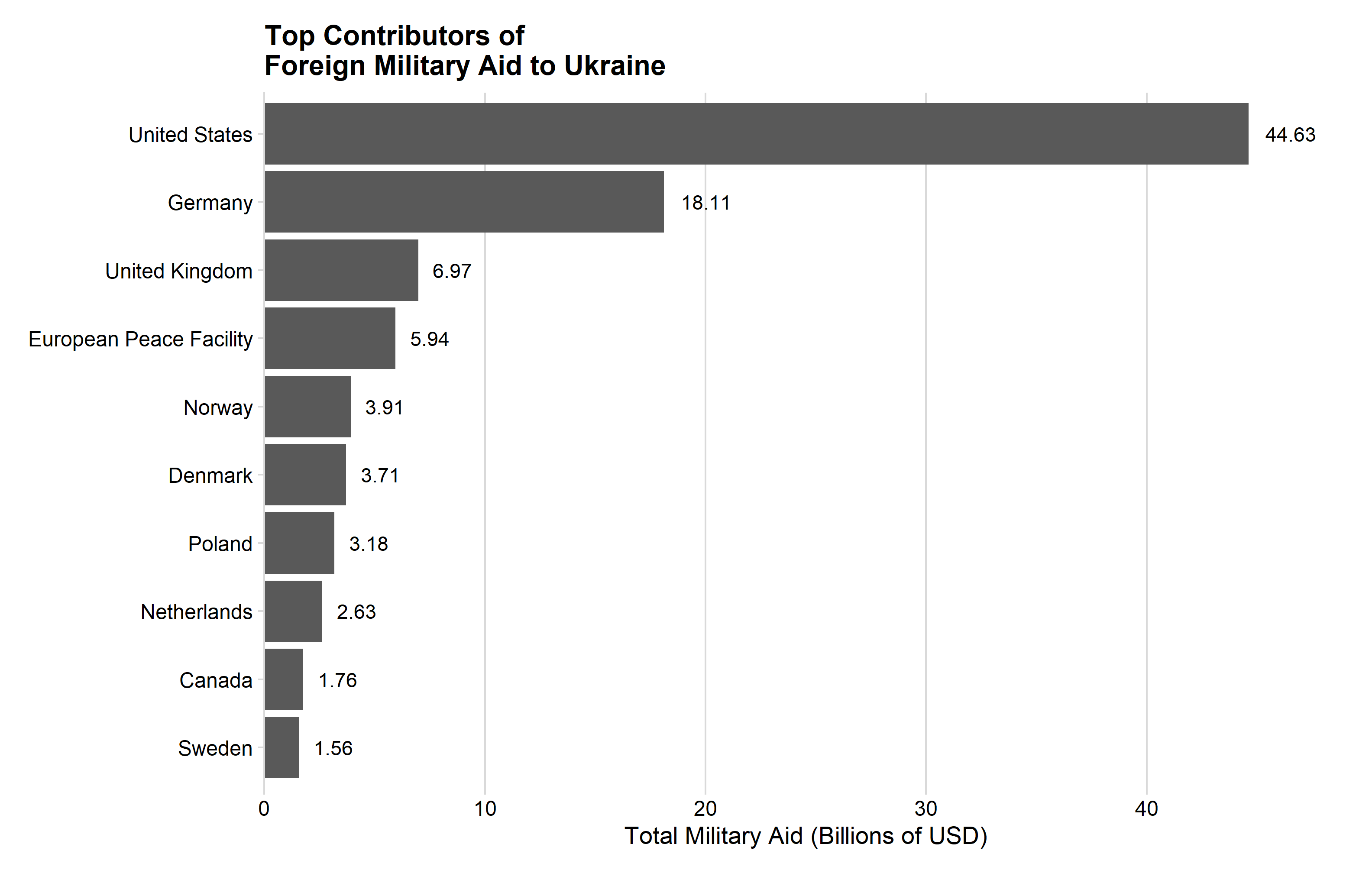
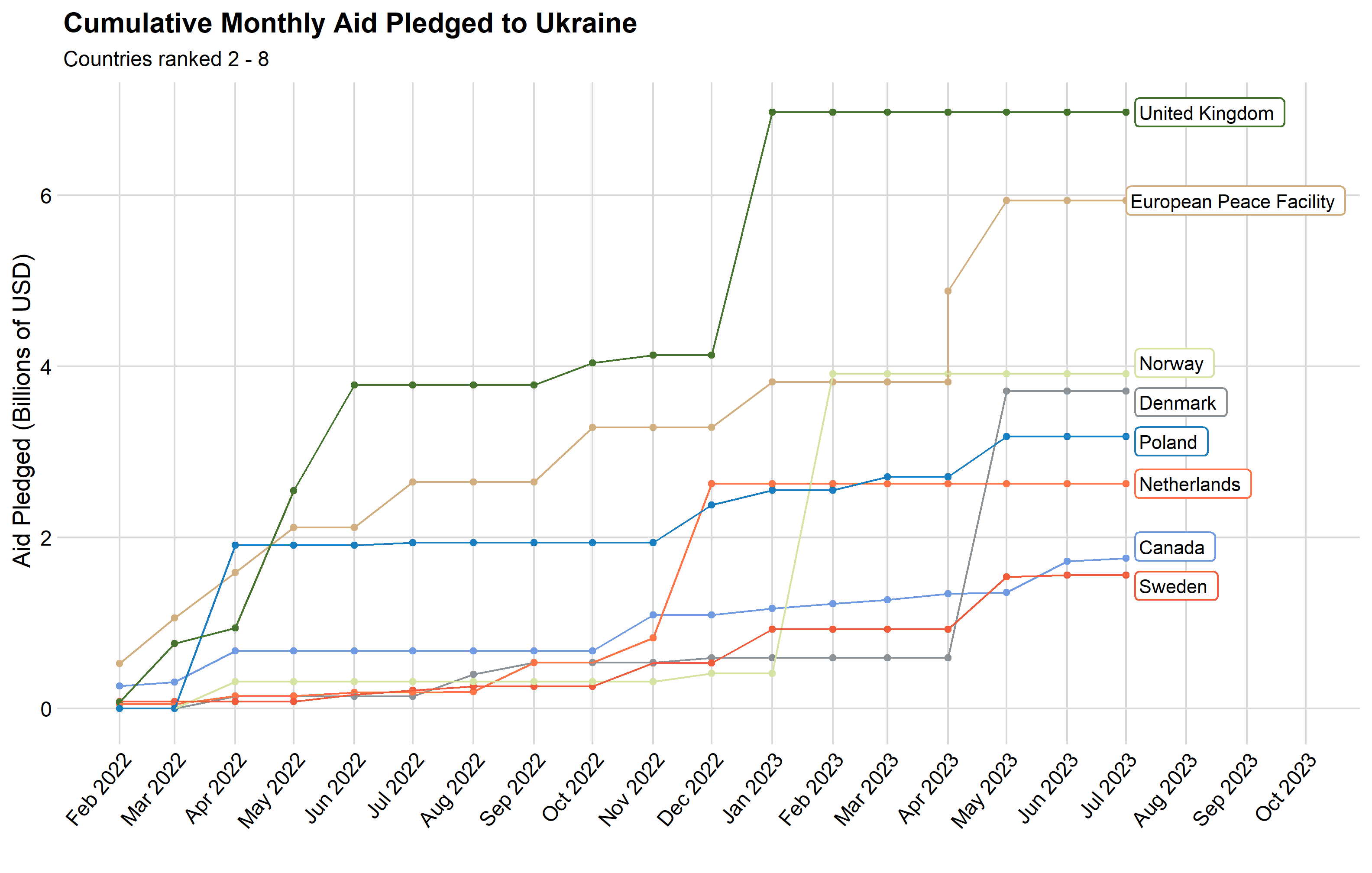
We will begin by painting a picture of the foreign aid that was submitted so that readers will have an idea of the aid timeline when looking at plots later on. We first highlighted the top ten contributors of military aid to Ukraine, including the United States, Germany, the UK, and more. Our team then compiled the monthly output of aid from these top ten countries to show a timeline of when aid was introduced into the conflict. Readers will notice significant jumps in funding in the beginning of the war (February to April 2022), followed by a gradual rate until the new year, when we see another large jump. The lack of funding in the most recent months of the war may be because several countries choose to follow the US’s lead. As American aid to Ukraine has slowed, so has aid from other countries, as illustrated in the third tab below. With the notable exception of the European Peace Facility, Norway, and Denmark, most countries’ aid pledges have leveled off alongside the US.
total_aid_bar %>%slice(33,12,34,23,8,24,21,5,31,35) %>%mutate(Countries =fct_reorder(Countries, Total_by_Country)) %>%mutate(val_lbl =paste0(" ", round(Total_by_Country, digits =2))) %>%ggplot()+geom_col(aes(x = Total_by_Country, y = Countries)) +geom_text(aes(x = Total_by_Country, y = Countries, label = val_lbl, hjust =-0.2), size =4)+labs(x ="Total Military Aid (Billions of USD)", y ="", title ="Top Contributors of \nForeign Military Aid to Ukraine")+theme_minimal_vgrid()+theme(legend.position ='none',plot.margin =unit(c(0.5, 0.5, 0.5, 0), "cm"))+scale_x_continuous(expand =expansion(mult =c(0, 0.1)))
Code
aid_col %>%mutate(Month =fct_inorder(Month, TRUE) %>%mdy()) %>%mutate(val_lbl =paste0(" ", round(monthly_total, digits =2))) %>%ggplot()+geom_col(aes(x = Month, y = monthly_total))+geom_text(aes(x = Month, y = monthly_total, label = val_lbl, vjust =-1), size =3)+labs(x ="", y ="Total Military Aid (Billions of USD)", title ="Cumulative Military Aid by Month", subtitle ="From Top Ten Contributing Countries")+theme_minimal_hgrid()+scale_x_date(date_labels ="%b %Y", date_breaks ="1 month", guide =guide_axis(angle =50))
Code
tam_df <- top_aid_months %>%mutate(Month =fct_inorder(Month, TRUE) %>%mdy()) %>%mutate(Cumulative = Cumulative /10^9) %>%mutate(Countries =ifelse(Countries =="United Kingdom", "Rest of Top Ten", Countries))tam_df %>%ggplot(aes(x = Month, y = Cumulative, group = Countries))+geom_point(aes(color = Countries))+geom_line(aes(color = Countries))+geom_label_repel(data =filter(tam_df, (Month ==mdy("7/1/2023")) & (Countries %in%c("United States", "Germany", "Rest of Top Ten"))), aes(color = Countries, label = Countries), hjust =-0,nudge_x =10, direction ="y", label.size =1,segment.color =NA ) +scale_color_simpsons() +geom_label_repel(data =filter(tam_df, (Month ==mdy("7/1/2023")) & (Countries %in%c("United States", "Germany", "Rest of Top Ten"))), aes(label = Countries), color ="black", hjust =-0,nudge_x =10, direction ="y", label.size =NA,segment.color =NA ) +labs(x ="",y ="Aid Pledged (Billions of USD)",title ="Cumulative Monthly Aid Pledged to Ukraine",subtitle ="By Top Ten Contributing Countries/Organizations")+theme_minimal_grid()+theme(legend.position ='none') +scale_x_date(date_labels ="%b %Y", date_breaks ="1 month", guide =guide_axis(angle =50))
Displayed in the chart below, a Ukrainian Military estimate of Russian Causalities over the course of the war is shown. With this chart, a clear escalation in casualties occurs especially after Week 17 of the war which is when the first major shipment of heavy weaponry was delivered from Germany.
Code
weekly <- russia_personnel %>%select(-POW,-`personnel*`) %>%mutate(week =floor_date(date, unit ="week"),daily_losses =c(NA, diff(personnel)),daily_losses_shifted =lead(daily_losses)) %>%group_by(week) %>%mutate(week_label =cur_group_id()) %>%group_by(week_label) %>%summarise(week_total =sum(daily_losses_shifted) ) %>%mutate(fill_color =ifelse(week_total <mean(week_total, na.rm =TRUE), "red", "blue")) %>%mutate(count_before =sum(week_label <17& fill_color =="blue", na.rm =TRUE),count_after =sum(week_label >=17& fill_color =="blue", na.rm =TRUE) ) %>%mutate(Week_Number = week_label,Week_Total = week_total )graph2 <- weekly %>%ggplot() +geom_bar(aes(x = Week_Number, y = Week_Total, fill = fill_color), stat ="identity", width =1) +theme_cowplot() +scale_fill_manual(values =c("red"="grey50", "blue"="red3")) +scale_x_continuous(expand =expand_scale(mult =c(0.01, 0.1))) +scale_y_continuous(labels = comma,expand =expand_scale(mult =c(0.03, 0.1))) +labs(x ="Week Number",y ="Weekly Total",title ="Ukrainian Estimates of Russian Personnel Casualities",caption ="Data up to Nov/26/2023" ) +geom_segment(x=(1), xend=(6), y=-100, yend =-100, color ='grey', linewidth =1, alpha =0.1) +geom_segment(x=(1), xend=(15), y=-700, yend =-700, color ='grey', linewidth =1, alpha =0.1) +geom_segment(x=(27), xend=(31), y=-100, yend =-100, color ='grey', linewidth =1, alpha =0.1) +geom_segment(x=(27), xend=(34), y=-700, yend =-700, color ='grey', linewidth =1, alpha =0.1) +geom_segment(x=(24), xend=(93), y=-1300, yend =-1300, color ='grey', linewidth =1, alpha =0.1) +annotate(geom ='text', x =6, y =-350,label ='Battle of Kyiv', size =3, color ='black') +annotate(geom ='text', x =8, y =-1000,label ='Siege of Mariupol', size =3, color ='black') +annotate(geom ='text', x =37, y =-350,label ='Kherson Counteroffensive', size =3, color ='black') +annotate(geom ='text', x =39, y =-1000,label ='Kharkiv Counteroffensive', size =3, color ='black') +annotate(geom ='text', x =45, y =-1650,label ='Battle of Bakhmut (Ongoing)', size =3, color ='black') +theme(plot.title =element_text(hjust =0, size =12),legend.position ="none")+geom_text(data =data.frame(x =30.5, y =7175, label =paste("Count Exceeding Mean Before 17 Weeks: ",weekly$count_before)),mapping =aes(x = x, y = y, label = label),inherit.aes =FALSE) +geom_text(data =data.frame(x =30.5, y =6720, label =paste("Count Exceeding Mean After 17 Weeks: ",weekly$count_after)),mapping =aes(x = x, y = y, label = label),inherit.aes =FALSE) +geom_hline(yintercept =mean(weekly$week_total, na.rm =TRUE),linetype ='dashed' ) +annotate('text', x =18, y =3750,color ='black', hjust =1,label ='Mean Casuality Estimates')ggplotly( graph2,tooltip =c("Week_Number","Week_Total"))
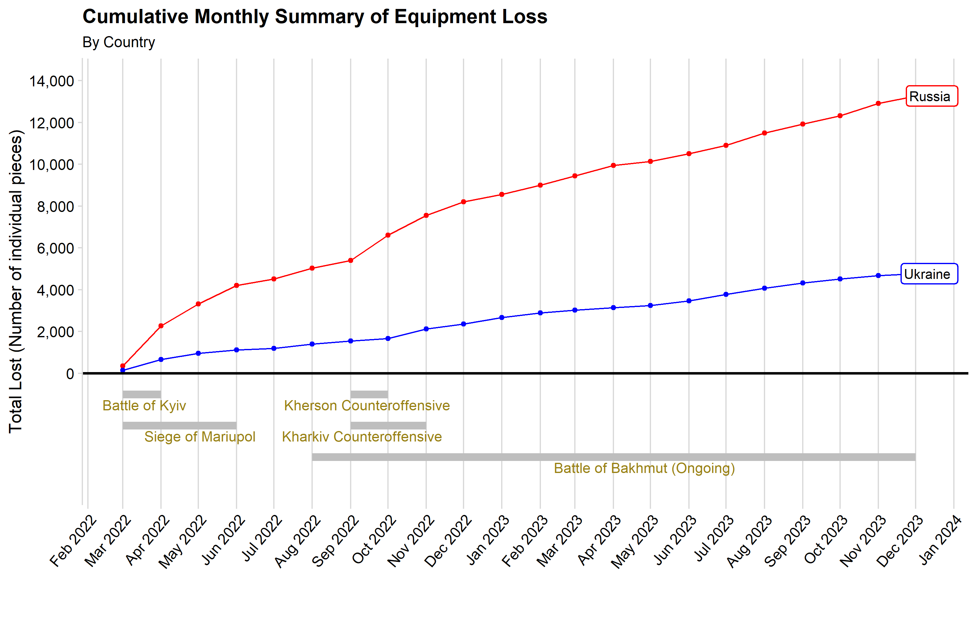
This chart illustrates the cumulative monthly summary of equipment loss for Russia and Ukraine from March 2022 to December 2023. The y-axis represents the total equipment loss values, encompassing various categories such as destroyed, abandoned, captured, and damaged pieces, while the x-axis denotes the timeline. The data provides crucial insights into the military dynamics of the conflict. Notably, the graph reveals a stark disparity in the impact on Russia’s and Ukraine’s equipment, with Russia experiencing significantly higher losses, particularly evident after the initial three months. After that period, Russia’s impacted equipment surpasses Ukraine’s by a considerable margin, reaching twice the number. This discrepancy sheds light on the differing degrees of resilience and adaptability demonstrated by the two nations in the face of the ongoing conflict.
Code
equip_summary_df <-read_csv(here("data_processed", "FilteredEquipSummaryByMonth.csv")) %>%mutate(Date =fct_inorder(Date, TRUE) %>%mdy()) %>%mutate(Country =str_to_title(Country))equip_summary_df %>%ggplot(aes(x = Date, y = Total_Values, color = Country, group = Country)) +geom_point() +geom_line() +geom_segment(x=mdy("3/1/2022"), xend=mdy("4/1/2022"), y=-1000, yend =-1000, color ='grey', linewidth =3) +geom_segment(x=mdy("3/1/2022"), xend=mdy("6/1/2022"), y=-2500, yend =-2500, color ='grey', linewidth =3) +geom_segment(x=mdy("9/1/2022"), xend=mdy("11/1/2022"), y=-2500, yend =-2500, color ='grey', linewidth =3) +geom_segment(x=mdy("9/1/2022"), xend=mdy("10/1/2022"), y=-1000, yend =-1000, color ='grey', linewidth =3) +geom_segment(x=mdy("8/1/2022"), xend=mdy("12/1/2023"), y=-4000, yend =-4000, color ='grey', linewidth =3) +annotate(geom ='text', x =mdy("6/1/2022"), y =-1500, hjust =1.6,label ='Battle of Kyiv', size =4, color ='#998114') +annotate(geom ='text', x =mdy("4/1/2022"), y =-3000, hjust =0.15,label ='Siege of Mariupol', size =4, color ='#998114') +annotate(geom ='text', x =mdy("9/1/2022"), y =-1500, hjust =0.4,label ='Kherson Counteroffensive', size =4, color ='#998114') +annotate(geom ='text', x =mdy("11/1/2022"), y =-3000, hjust =0.9,label ='Kharkiv Counteroffensive', size =4, color ='#998114') +annotate(geom ='text', x =mdy("12/1/2022"), y =-4500, hjust =-0.5,label ='Battle of Bakhmut (Ongoing)', size =4, color ='#998114') +geom_hline(aes(yintercept =0), color ='black', size =1) +geom_label_repel(data =filter(equip_summary_df, Date ==mdy("12/1/2023")), aes(color = Country, label = Country), hjust =-0,nudge_x =10, direction ="y", label.size =1,segment.color =NA ) +scale_color_manual(values =c("Russia"="red", "Ukraine"="blue")) +geom_label_repel(data =filter(equip_summary_df, Date ==mdy("12/1/2023")), aes(label = Country), color ="black", hjust =-0,nudge_x =10, direction ="y", label.size =NA,segment.color =NA ) +labs(x ="",y ="Total Lost (Number of individual pieces)",title ="Cumulative Monthly Summary of Equipment Loss",subtitle ="By Country",caption ="" ) +scale_y_continuous(breaks =seq(round(min(equip_summary_df$Total_Values), digits =-3), round(max(equip_summary_df$Total_Values) +2000, digits =-3), by =2000),labels = comma,expand =expand_scale(mult =c(0.1, 0.1)) ) +scale_x_date(date_labels ="%b %Y", date_breaks ="1 month", guide =guide_axis(angle =50)) +theme_minimal_vgrid() +theme(legend.position ='none')
Tanks
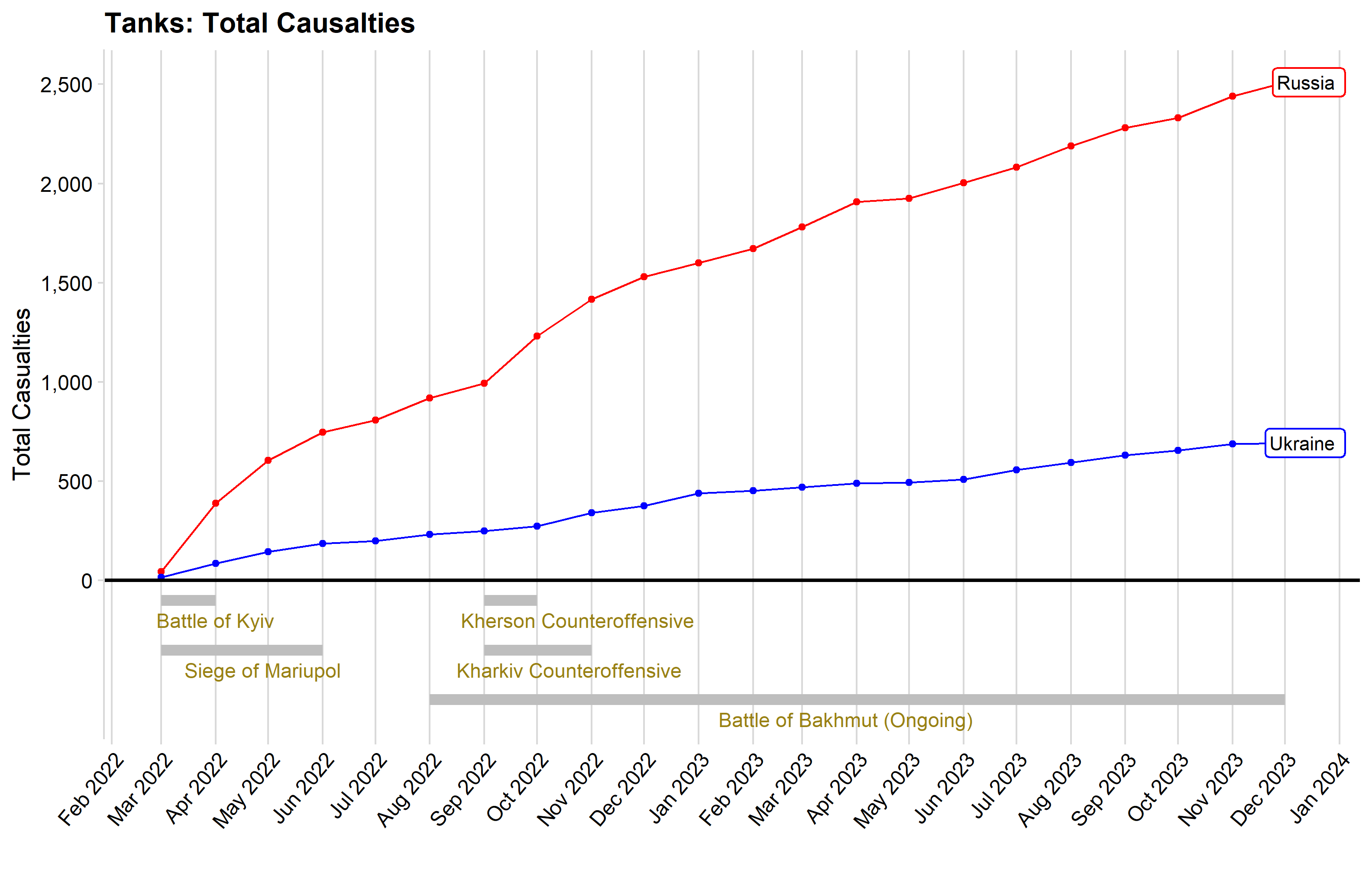
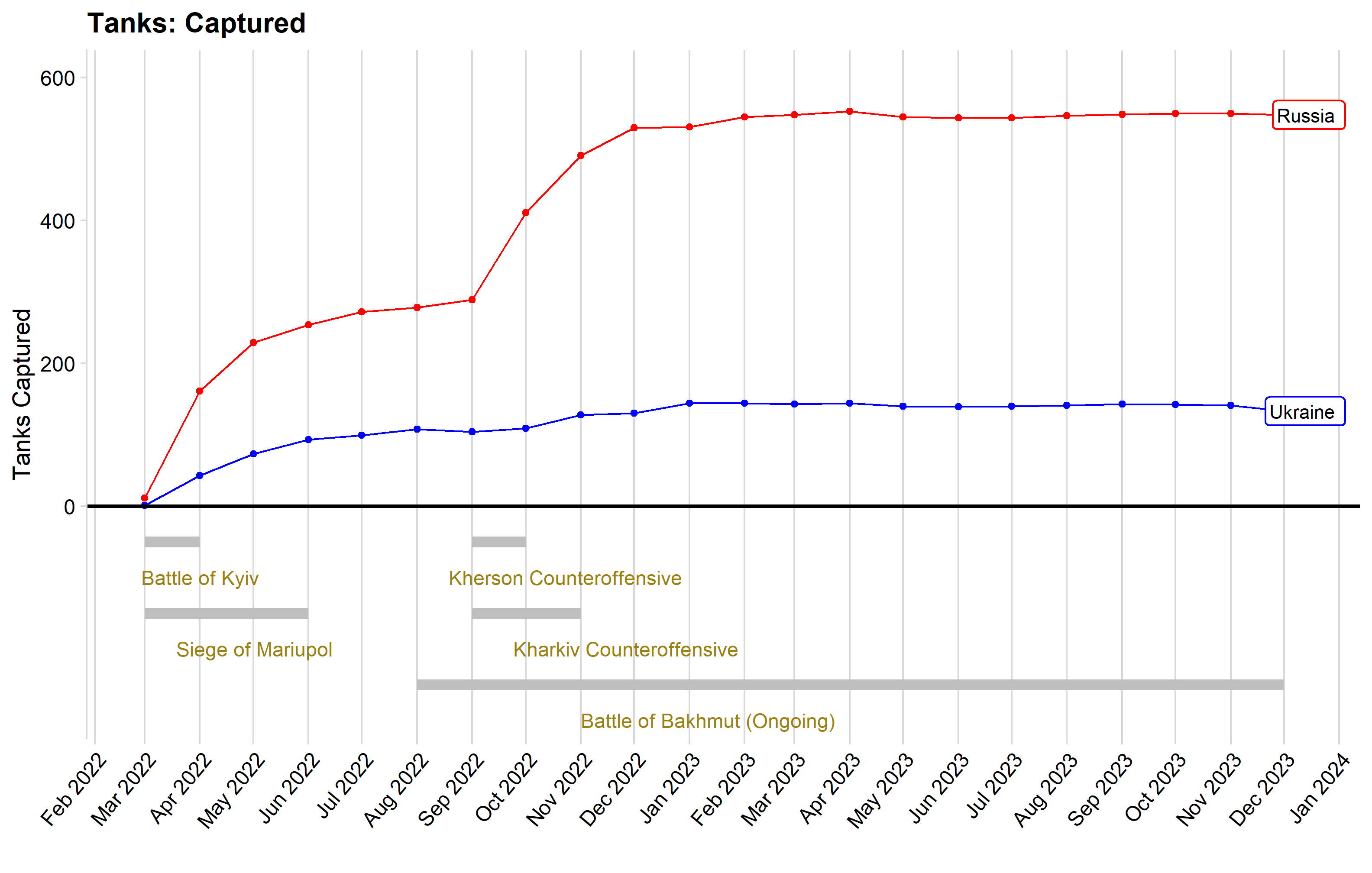
The below charts show the differences between Russian and Ukrainian tank casualties over the course of the war. The first four charts show cumulative losses. The majority of tank casualties are from destroyed tanks, but Russia has also had many of their tanks either captured or abandoned.
There is a rather sharp slope to Russia’s casualties at the beginning of the war, corresponding with not only the Battle of Kyiv and Siege of Mariupol, but also with the large amounts of aid that were pledged within the first few months of the war. There was also a huge increase of captured Russian tanks from 9/1/2022 through 11/1/2022. This corresponds with a plateau in aid from the international community. This may indicate that Ukraine was trying to capture tanks for their own use instead of destroying them due to their lack of purchasing power/inventory. Alternatively, it may be because of the Russian’s over extension into Ukraine and the lack of supply lines needed for refueling during the Kharkiv and Kherson Counteroffensives. As you can see in the final tab “Confirmed Tank Casualties”, the chart compares the data to the mean to determine if a certain week exceeded the mean or not. This count starts at week 17 of the war as this is when the first notable heavy military equipment has been delierved to Ukraine.
It should be noted that while there was a steep increase in aid at the beginning of 2023, the slope of both countries casualties stayed relatively constant. This indicates that either funding to the Ukraine was needed just to keep pace with Russia, or the aid was being used in other forms of combat.
tanks_df <- tanks %>%mutate(Date =fct_inorder(Date, TRUE) %>%mdy())tanks_df %>%ggplot(aes(x = Date, y = type_total, color = country, group = country))+geom_point()+geom_line()+geom_segment(x=mdy("3/1/2022"), xend=mdy("4/1/2022"), y=-100, yend =-100, color ='grey', linewidth =3) +geom_segment(x=mdy("3/1/2022"), xend=mdy("6/1/2022"), y=-350, yend =-350, color ='grey', linewidth =3) +geom_segment(x=mdy("9/1/2022"), xend=mdy("11/1/2022"), y=-350, yend =-350, color ='grey', linewidth =3) +geom_segment(x=mdy("9/1/2022"), xend=mdy("10/1/2022"), y=-100, yend =-100, color ='grey', linewidth =3) +geom_segment(x=mdy("8/1/2022"), xend=mdy("12/1/2023"), y=-600, yend =-600, color ='grey', linewidth =3) +annotate(geom ='text', x =mdy("5/1/2022"), y =-200, hjust =0.95,label ='Battle of Kyiv', size =4, color ='#998114') +annotate(geom ='text', x =mdy("4/1/2022"), y =-450, hjust =0.2,label ='Siege of Mariupol', size =4, color ='#998114') +annotate(geom ='text', x =mdy("9/1/2022"), y =-200, hjust =0.1,label ='Kherson Counteroffensive', size =4, color ='#998114') +annotate(geom ='text', x =mdy("11/1/2022"), y =-450, hjust =0.6,label ='Kharkiv Counteroffensive', size =4, color ='#998114') +annotate(geom ='text', x =mdy("11/1/2022"), y =-700, hjust =-0.5,label ='Battle of Bakhmut (Ongoing)', size =4, color ='#998114') +geom_hline(aes(yintercept =0), color ='black', size =1) +geom_label_repel(data =filter(tanks_df, Date ==mdy("12/1/2023")), aes(color = country, label = country), hjust =-0,nudge_x =10, direction ="y", label.size =1,segment.color =NA ) +scale_color_manual(values =c("Russia"="red", "Ukraine"="blue")) +geom_label_repel(data =filter(tanks_df, Date ==mdy("12/1/2023")), aes(label = country), color ="black", hjust =-0,nudge_x =10, direction ="y", label.size =NA,segment.color =NA ) +labs(x ="", y ="Total Casualties", title ="Tanks: Total Causalties") +scale_x_date(guide =guide_axis(angle =50), date_labels ="%b %Y", date_breaks ="1 month") +scale_y_continuous(breaks =seq(round(min(tanks_df$type_total), digits =-2), round(max(tanks_df$type_total), digits =-2), by =500),labels = comma,expand =expansion(mult =c(0.03, 0.05)) ) +theme_minimal_vgrid()+theme(legend.position ='none')
Code
tanks_df <- tanks %>%mutate(Date =fct_inorder(Date, TRUE) %>%mdy())tanks_df %>%ggplot(aes(x = Date, y = destroyed, color = country, group = country))+geom_point()+geom_line()+geom_segment(x=mdy("3/1/2022"), xend=mdy("4/1/2022"), y=-100, yend =-100, color ='grey', linewidth =3) +geom_segment(x=mdy("3/1/2022"), xend=mdy("6/1/2022"), y=-350, yend =-350, color ='grey', linewidth =3) +geom_segment(x=mdy("9/1/2022"), xend=mdy("11/1/2022"), y=-350, yend =-350, color ='grey', linewidth =3) +geom_segment(x=mdy("9/1/2022"), xend=mdy("10/1/2022"), y=-100, yend =-100, color ='grey', linewidth =3) +geom_segment(x=mdy("8/1/2022"), xend=mdy("12/1/2023"), y=-600, yend =-600, color ='grey', linewidth =3) +annotate(geom ='text', x =mdy("5/1/2022"), y =-200, hjust =0.95,label ='Battle of Kyiv', size =4, color ='#998114') +annotate(geom ='text', x =mdy("4/1/2022"), y =-450, hjust =0.15,label ='Siege of Mariupol', size =4, color ='#998114') +annotate(geom ='text', x =mdy("9/1/2022"), y =-200, hjust =0.1,label ='Kherson Counteroffensive', size =4, color ='#998114') +annotate(geom ='text', x =mdy("11/1/2022"), y =-450, hjust =0.3,label ='Kharkiv Counteroffensive', size =4, color ='#998114') +annotate(geom ='text', x =mdy("11/1/2022"), y =-700, hjust =0,label ='Battle of Bakhmut (Ongoing)', size =4, color ='#998114') +geom_hline(aes(yintercept =0), color ='black', size =1) +geom_label_repel(data =filter(tanks_df, Date ==mdy("12/1/2023")), aes(color = country, label = country), hjust =-0,nudge_x =10, direction ="y", label.size =1,segment.color =NA ) +scale_color_manual(values =c("Russia"="red", "Ukraine"="blue")) +geom_label_repel(data =filter(tanks_df, Date ==mdy("12/1/2023")), aes(label = country), color ="black", hjust =-0,nudge_x =10, direction ="y", label.size =NA,segment.color =NA ) +labs(x ="", y ="Tanks Destroyed", title ="Tanks: Destroyed")+scale_x_date(guide =guide_axis(angle =50), date_labels ="%b %Y", date_breaks ="1 month") +scale_y_continuous(breaks =seq(round(min(tanks_df$destroyed), digits =-2), round(max(tanks_df$destroyed), digits =-2), by =500),labels = comma,expand =expansion(mult =c(0.03, 0.05)) ) +theme_minimal_vgrid()+theme(legend.position ='none')
Code
tanks_df <- tanks %>%mutate(Date =fct_inorder(Date, TRUE) %>%mdy())tanks_df %>%ggplot(aes(x = Date, y = captured, color = country, group = country))+geom_point()+geom_line()+geom_segment(x=mdy("3/1/2022"), xend=mdy("4/1/2022"), y=-50, yend =-50, color ='grey', linewidth =3) +geom_segment(x=mdy("3/1/2022"), xend=mdy("6/1/2022"), y=-150, yend =-150, color ='grey', linewidth =3) +geom_segment(x=mdy("9/1/2022"), xend=mdy("11/1/2022"), y=-150, yend =-150, color ='grey', linewidth =3) +geom_segment(x=mdy("9/1/2022"), xend=mdy("10/1/2022"), y=-50, yend =-50, color ='grey', linewidth =3) +geom_segment(x=mdy("8/1/2022"), xend=mdy("12/1/2023"), y=-250, yend =-250, color ='grey', linewidth =3) +annotate(geom ='text', x =mdy("5/1/2022"), y =-100, hjust =0.95,label ='Battle of Kyiv', size =4, color ='#998114') +annotate(geom ='text', x =mdy("4/1/2022"), y =-200, hjust =0.15,label ='Siege of Mariupol', size =4, color ='#998114') +annotate(geom ='text', x =mdy("9/1/2022"), y =-100, hjust =0.1,label ='Kherson Counteroffensive', size =4, color ='#998114') +annotate(geom ='text', x =mdy("11/1/2022"), y =-200, hjust =0.3,label ='Kharkiv Counteroffensive', size =4, color ='#998114') +annotate(geom ='text', x =mdy("11/1/2022"), y =-300, hjust =0,label ='Battle of Bakhmut (Ongoing)', size =4, color ='#998114') +geom_hline(aes(yintercept =0), color ='black', size =1) +geom_label_repel(data =filter(tanks_df, Date ==mdy("12/1/2023")), aes(color = country, label = country), hjust =-0,nudge_x =10, direction ="y", label.size =1,segment.color =NA ) +scale_color_manual(values =c("Russia"="red", "Ukraine"="blue")) +scale_y_continuous(labels =c(0,500), breaks =c(0,500))+geom_label_repel(data =filter(tanks_df, Date ==mdy("12/1/2023")), aes(label = country), color ="black", hjust =-0,nudge_x =10, direction ="y", label.size =NA,segment.color =NA ) +labs(x ="", y ="Tanks Captured", title ="Tanks: Captured")+scale_x_date(guide =guide_axis(angle =50), date_labels ="%b %Y", date_breaks ="1 month") +scale_y_continuous(breaks =seq(round(min(tanks_df$captured), digits =-2), round(max(tanks_df$captured), digits =-2), by =200),labels = comma,expand =expansion(mult =c(0.03, 0.1)) ) +theme_minimal_vgrid()+theme(legend.position ='none')
Code
tanks_df <- tanks %>%mutate(Date =fct_inorder(Date, TRUE) %>%mdy())tanks_df %>%ggplot(aes(x = Date, y = abandoned, color = country, group = country))+geom_point()+geom_line()+geom_segment(x=mdy("3/1/2022"), xend=mdy("4/1/2022"), y=-20, yend =-20, color ='grey', linewidth =3) +geom_segment(x=mdy("3/1/2022"), xend=mdy("6/1/2022"), y=-40, yend =-40, color ='grey', linewidth =3) +geom_segment(x=mdy("9/1/2022"), xend=mdy("11/1/2022"), y=-40, yend =-40, color ='grey', linewidth =3) +geom_segment(x=mdy("9/1/2022"), xend=mdy("10/1/2022"), y=-20, yend =-20, color ='grey', linewidth =3) +geom_segment(x=mdy("8/1/2022"), xend=mdy("12/1/2023"), y=-60, yend =-60, color ='grey', linewidth =3) +annotate(geom ='text', x =mdy("5/1/2022"), y =-30, hjust =0.95,label ='Battle of Kyiv', size =4, color ='#998114') +annotate(geom ='text', x =mdy("4/1/2022"), y =-50, hjust =0.15,label ='Siege of Mariupol', size =4, color ='#998114') +annotate(geom ='text', x =mdy("9/1/2022"), y =-30, hjust =0.1,label ='Kherson Counteroffensive', size =4, color ='#998114') +annotate(geom ='text', x =mdy("11/1/2022"), y =-50, hjust =0.3,label ='Kharkiv Counteroffensive', size =4, color ='#998114') +annotate(geom ='text', x =mdy("11/1/2022"), y =-70, hjust =0,label ='Battle of Bakhmut (Ongoing)', size =4, color ='#998114') +geom_hline(aes(yintercept =0), color ='black', size =1) +geom_label_repel(data =filter(tanks_df, Date ==mdy("12/1/2023")), aes(color = country, label = country), hjust =-0,nudge_x =10, direction ="y", label.size =1,segment.color =NA ) +scale_color_manual(values =c("Russia"="red", "Ukraine"="blue")) +geom_label_repel(data =filter(tanks_df, Date ==mdy("12/1/2023")), aes(label = country), color ="black", hjust =-0,nudge_x =10, direction ="y", label.size =NA,segment.color =NA ) +labs(x ="", y ="Tanks Abandoned", title ="Tanks: Abandoned")+scale_x_date(date_labels ="%b %Y", date_breaks ="1 month", guide =guide_axis(angle =50)) +scale_y_continuous(breaks =seq(round(min(tanks_df$abandoned), digits =-2), round(max(tanks_df$abandoned), digits =-2), by =50),labels = comma,expand =expansion(mult =c(0.03, 0.1)) ) +theme_minimal_vgrid()+theme(legend.position ='none')
Code
weekly_tank <- russia_equipment %>%select(date,day,tank) %>%mutate(week =floor_date(date, unit ="week"),daily_losses =c(NA, diff(tank)),daily_losses_shifted =lead(daily_losses)) %>%group_by(week) %>%mutate(week_label =cur_group_id()) %>%group_by(week_label) %>%summarise(week_total =sum(daily_losses_shifted) ) %>%mutate(fill_color =ifelse(week_total <mean(week_total, na.rm =TRUE), "red", "blue")) %>%mutate(count_before =sum(week_label <17& fill_color =="blue", na.rm =TRUE),count_after =sum(week_label >=17& fill_color =="blue", na.rm =TRUE)) %>%mutate(Week_Number = week_label,Week_Total = week_total )graph1 <- weekly_tank %>%ggplot() +geom_bar(aes(x = Week_Number, y = Week_Total, fill = fill_color), stat ="identity", width =1) +theme_cowplot() +scale_fill_manual(values =c("red"="grey50", "blue"="red3")) +scale_x_continuous(expand =expand_scale(mult =c(0.01, 0.1))) +scale_y_continuous(labels = comma,expand =expand_scale(mult =c(0.03, 0.1))) +labs(x ="Week Number",y ="Weekly Total",title ="Confirmed Russian Tank Casualities",caption ="Data up to Nov/26/2023" ) +geom_segment(x=(1), xend=(6), y=-5, yend =-5, color ='grey', linewidth =1, alpha =0.1) +geom_segment(x=(1), xend=(15), y=-16, yend =-16, color ='grey', linewidth =1, alpha =0.1) +geom_segment(x=(27), xend=(31), y=-5, yend =-5, color ='grey', linewidth =1, alpha =0.1) +geom_segment(x=(27), xend=(34), y=-16, yend =-16, color ='grey', linewidth =1, alpha =0.1) +geom_segment(x=(24), xend=(93), y=-27, yend =-27, color ='grey', linewidth =1, alpha =0.1) +annotate(geom ='text', x =6, y =-11,label ='Battle of Kyiv', size =3, color ='black') +annotate(geom ='text', x =8, y =-22,label ='Siege of Mariupol', size =3, color ='black') +annotate(geom ='text', x =37, y =-10,label ='Kherson Counteroffensive', size =3, color ='black') +annotate(geom ='text', x =39, y =-22,label ='Kharkiv Counteroffensive', size =3, color ='black') +annotate(geom ='text', x =45, y =-33,label ='Battle of Bakhmut (Ongoing)', size =3, color ='black') +geom_hline(aes(yintercept =0), color ='black', size =1) +theme(plot.title =element_text(hjust =0),legend.position ="none") +geom_text(data =data.frame(x =60, y =160, label =paste("Count Exceeding Mean Before 17 Weeks: ",weekly_tank$count_before)),mapping =aes(x = x, y = y, label = label),inherit.aes =FALSE) +geom_text(data =data.frame(x =60, y =150, label =paste("Count Exceeding Mean After 17 Weeks: ",weekly_tank$count_after)),mapping =aes(x = x, y = y, label = label),inherit.aes =FALSE, ) +geom_hline(yintercept =mean(weekly_tank$week_total, na.rm =TRUE),color ='black',linetype ='dashed' ) +annotate('text', x =45, y =59,color ='black', hjust =1,label ='Mean Tank\n Casualities',size =3)ggplotly(graph1 ,tooltip =c("Week_Number","Week_Total"))
Aircraft
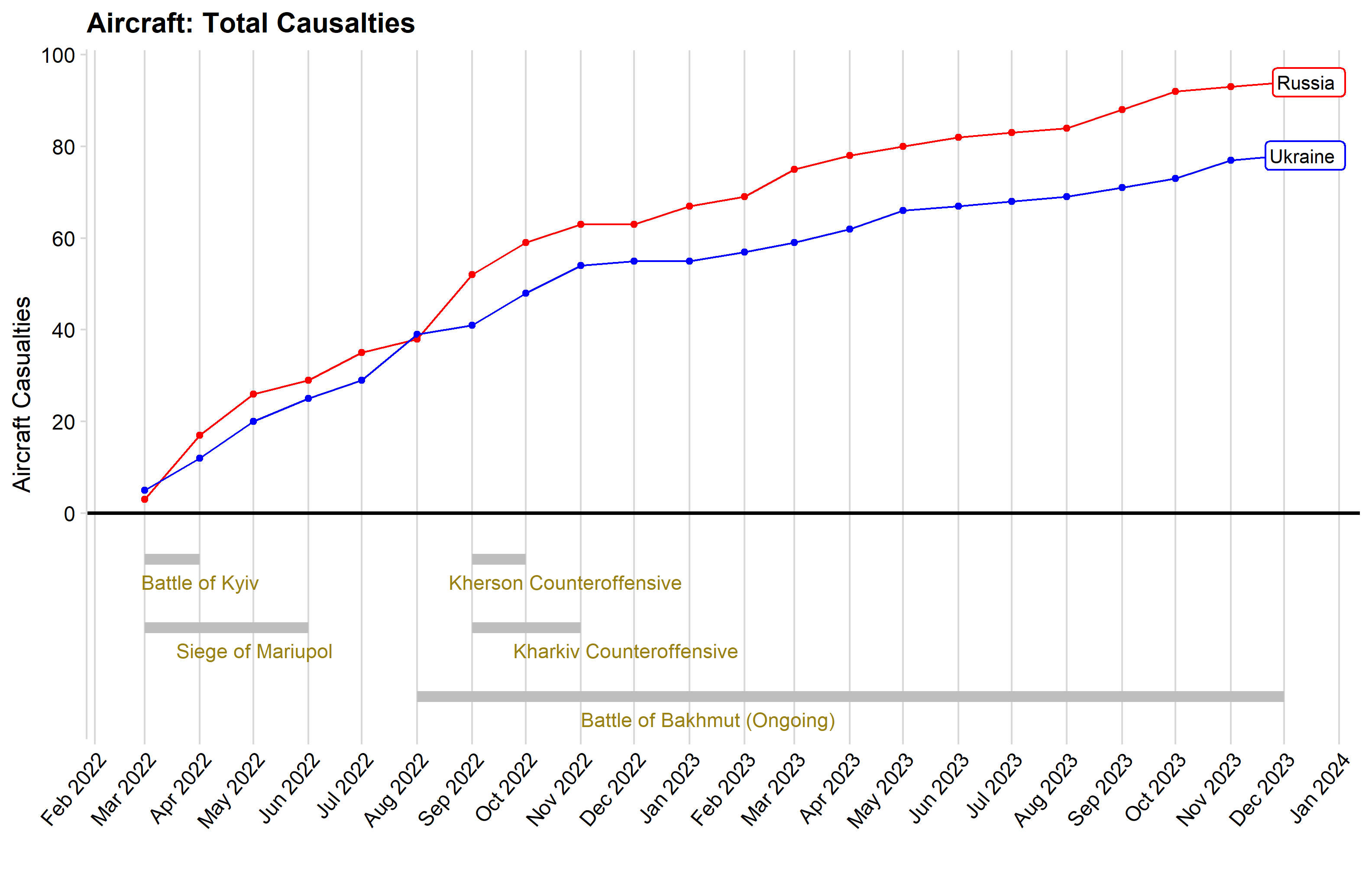
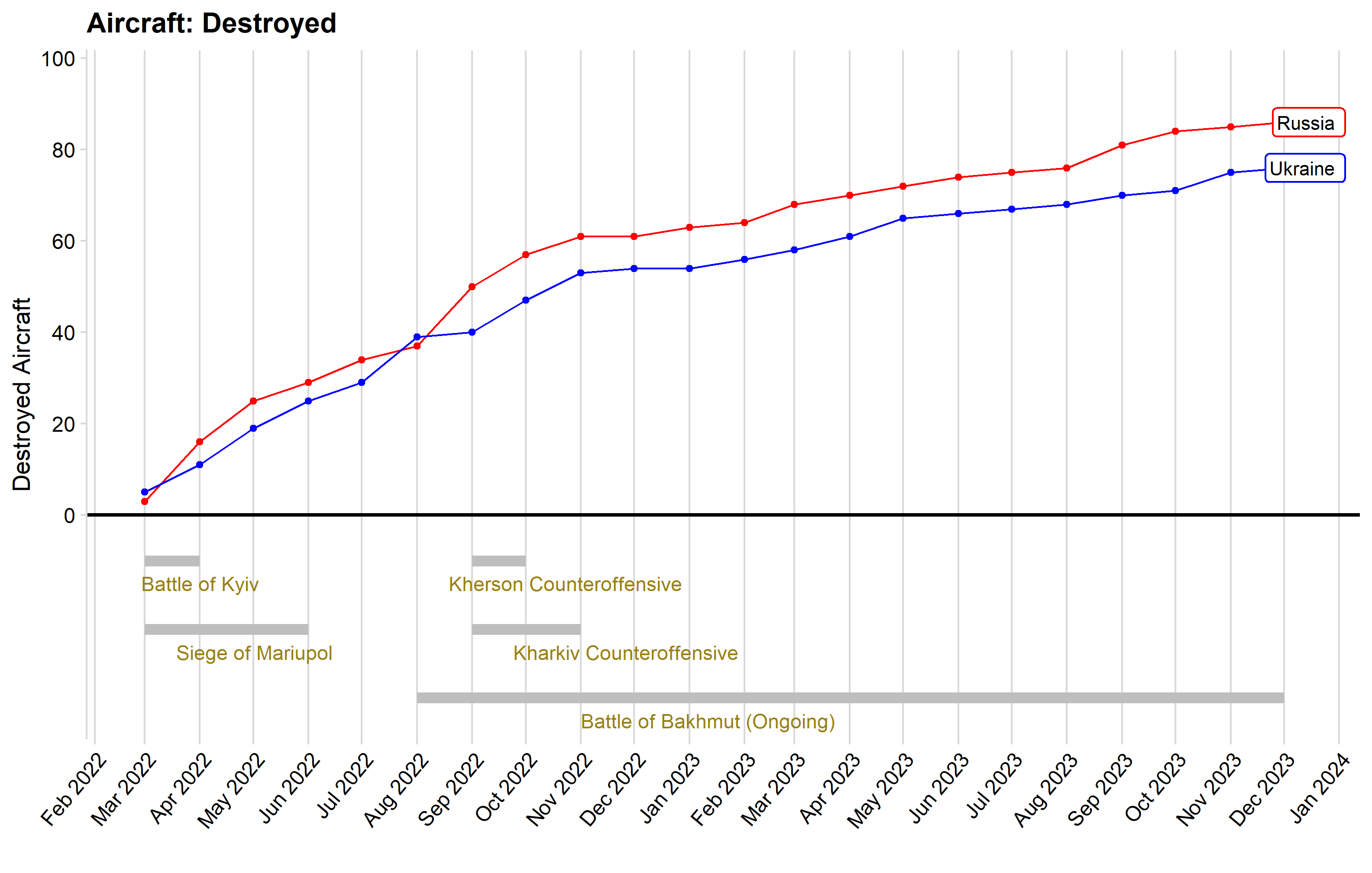
The following graphs illustrate the difference between cumulative Russian and Ukrainian aircraft casualties. The non-helicopter plots show a much closer war than the tank plots. In fact, our team would make the assumption that Russia is winning the aerial battle in terms of percentage of aircraft fleets lost, but we do not have access to the inventory of either country’s fleets at the beginning of the invasion.
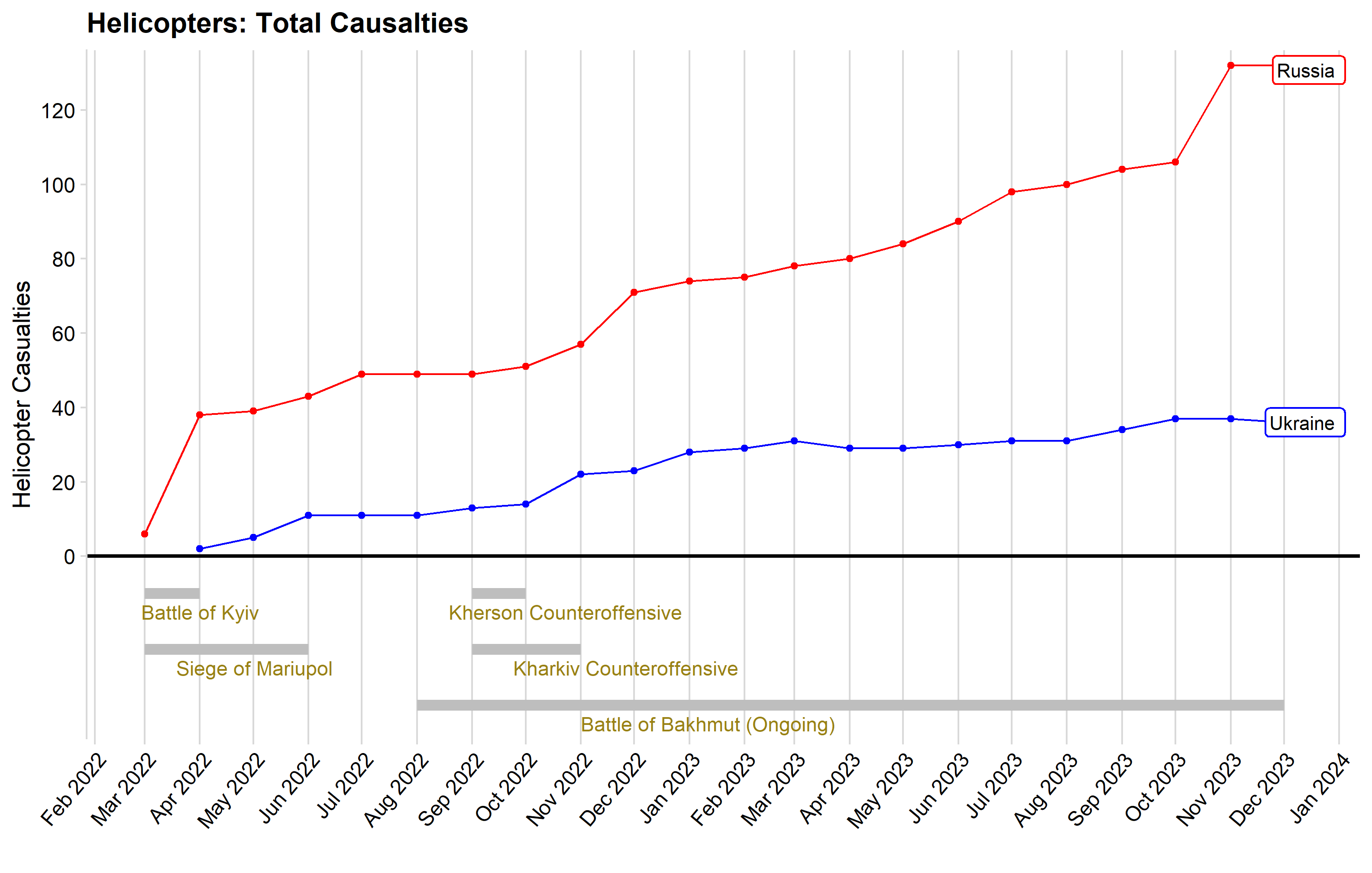
Russia faced huge helicopter casualties in the first 2 months of the war. Nearly 33% of their helicopter casualties occurred during these months. Again, this corresponds to the huge amounts of aid that were pledged in the first months, as well as the Battle of Kyiv and Siege of Mariupol. Russia also faced a steep increase in helicopter casualties during October this year. Unfortunately, our aid data set only goes through July this year, so we cannot attribute these casualties directly to aid. However, we can infer from news sources that Ukrainian troops have become more and more effective with their donated weapon systems, to include the US-made Patriot missile system. This would account for the dramatic increase of destroyed Russian helicopters.
These graphs illustrate a quick start to the war in terms of aircraft casualties, corresponding with aid pledges and the Battle of Kyiv and the Siege of Mariupol. Non-helicopter aircraft casualties have been relatively consistent month over month since 9/1/2022, but helicopter casualties for Russia continue to grow at an alarming rate.
aircraft_df <- aircraft %>%mutate(Date =fct_inorder(Date, TRUE) %>%mdy())aircraft_df %>%ggplot(aes(x = Date, y = type_total, color = country, group = country))+geom_point()+geom_line()+geom_segment(x=mdy("3/1/2022"), xend=mdy("4/1/2022"), y=-10, yend =-10, color ='grey', linewidth =3) +geom_segment(x=mdy("3/1/2022"), xend=mdy("6/1/2022"), y=-25, yend =-25, color ='grey', linewidth =3) +geom_segment(x=mdy("9/1/2022"), xend=mdy("11/1/2022"), y=-25, yend =-25, color ='grey', linewidth =3) +geom_segment(x=mdy("9/1/2022"), xend=mdy("10/1/2022"), y=-10, yend =-10, color ='grey', linewidth =3) +geom_segment(x=mdy("8/1/2022"), xend=mdy("12/1/2023"), y=-40, yend =-40, color ='grey', linewidth =3) +annotate(geom ='text', x =mdy("5/1/2022"), y =-15, hjust =0.95,label ='Battle of Kyiv', size =4, color ='#998114') +annotate(geom ='text', x =mdy("4/1/2022"), y =-30, hjust =0.15,label ='Siege of Mariupol', size =4, color ='#998114') +annotate(geom ='text', x =mdy("9/1/2022"), y =-15, hjust =0.1,label ='Kherson Counteroffensive', size =4, color ='#998114') +annotate(geom ='text', x =mdy("11/1/2022"), y =-30, hjust =0.3,label ='Kharkiv Counteroffensive', size =4, color ='#998114') +annotate(geom ='text', x =mdy("11/1/2022"), y =-45, hjust =0,label ='Battle of Bakhmut (Ongoing)', size =4, color ='#998114') +geom_hline(aes(yintercept =0), color ='black', size =1) +geom_label_repel(data =filter(aircraft_df, Date ==mdy("12/1/2023")), aes(color = country, label = country), hjust =-0,nudge_x =10, direction ="y", label.size =1,segment.color =NA ) +scale_color_manual(values =c("Russia"="red", "Ukraine"="blue")) +geom_label_repel(data =filter(aircraft_df, Date ==mdy("12/1/2023")), aes(label = country), color ="black", hjust =-0,nudge_x =10, direction ="y", label.size =NA,segment.color =NA ) +labs(x ="", y ="Aircraft Casualties", title ="Aircraft: Total Causalties")+scale_x_date(date_labels ="%b %Y", date_breaks ="1 month", guide =guide_axis(angle =50)) +scale_y_continuous(breaks =seq(round(min(aircraft_df$type_total), digits =-1), round(max(aircraft_df$type_total), digits =-2), by =20),expand =expansion(mult =c(0.03, 0.05)) ) +theme_minimal_vgrid()+theme(legend.position ='none')
Code
aircraft_df <- aircraft %>%mutate(Date =fct_inorder(Date, TRUE) %>%mdy())aircraft_df %>%ggplot(aes(x = Date, y = destroyed, color = country, group = country))+geom_point()+geom_line()+geom_segment(x=mdy("3/1/2022"), xend=mdy("4/1/2022"), y=-10, yend =-10, color ='grey', linewidth =3) +geom_segment(x=mdy("3/1/2022"), xend=mdy("6/1/2022"), y=-25, yend =-25, color ='grey', linewidth =3) +geom_segment(x=mdy("9/1/2022"), xend=mdy("11/1/2022"), y=-25, yend =-25, color ='grey', linewidth =3) +geom_segment(x=mdy("9/1/2022"), xend=mdy("10/1/2022"), y=-10, yend =-10, color ='grey', linewidth =3) +geom_segment(x=mdy("8/1/2022"), xend=mdy("12/1/2023"), y=-40, yend =-40, color ='grey', linewidth =3) +annotate(geom ='text', x =mdy("5/1/2022"), y =-15, hjust =0.95,label ='Battle of Kyiv', size =4, color ='#998114') +annotate(geom ='text', x =mdy("4/1/2022"), y =-30, hjust =0.15,label ='Siege of Mariupol', size =4, color ='#998114') +annotate(geom ='text', x =mdy("9/1/2022"), y =-15, hjust =0.1,label ='Kherson Counteroffensive', size =4, color ='#998114') +annotate(geom ='text', x =mdy("11/1/2022"), y =-30, hjust =0.3,label ='Kharkiv Counteroffensive', size =4, color ='#998114') +annotate(geom ='text', x =mdy("11/1/2022"), y =-45, hjust =0,label ='Battle of Bakhmut (Ongoing)', size =4, color ='#998114') +geom_hline(aes(yintercept =0), color ='black', size =1) +geom_label_repel(data =filter(aircraft_df, Date ==mdy("12/1/2023")), aes(color = country, label = country), hjust =-0,nudge_x =10, direction ="y", label.size =1,segment.color =NA ) +scale_color_manual(values =c("Russia"="red", "Ukraine"="blue")) +geom_label_repel(data =filter(aircraft_df, Date ==mdy("12/1/2023")), aes(label = country), color ="black", hjust =-0,nudge_x =10, direction ="y", label.size =NA,segment.color =NA ) +labs(x ="", y ="Destroyed Aircraft", title ="Aircraft: Destroyed")+scale_x_date(date_labels ="%b %Y", date_breaks ="1 month", guide =guide_axis(angle =50)) +scale_y_continuous(breaks =seq(round(min(aircraft_df$destroyed), digits =-1), round(max(aircraft_df$destroyed), digits =-2), by =20),expand =expansion(mult =c(0.03, 0.12)) ) +theme_minimal_vgrid()+theme(legend.position ='none')
Code
helicopters_df <- helicopters %>%mutate(Date =fct_inorder(Date, TRUE) %>%mdy())helicopters_df %>%ggplot(aes(x = Date, y = type_total, color = country, group = country))+geom_point()+geom_line()+geom_segment(x=mdy("3/1/2022"), xend=mdy("4/1/2022"), y=-10, yend =-10, color ='grey', linewidth =3) +geom_segment(x=mdy("3/1/2022"), xend=mdy("6/1/2022"), y=-25, yend =-25, color ='grey', linewidth =3) +geom_segment(x=mdy("9/1/2022"), xend=mdy("11/1/2022"), y=-25, yend =-25, color ='grey', linewidth =3) +geom_segment(x=mdy("9/1/2022"), xend=mdy("10/1/2022"), y=-10, yend =-10, color ='grey', linewidth =3) +geom_segment(x=mdy("8/1/2022"), xend=mdy("12/1/2023"), y=-40, yend =-40, color ='grey', linewidth =3) +annotate(geom ='text', x =mdy("5/1/2022"), y =-15, hjust =0.95,label ='Battle of Kyiv', size =4, color ='#998114') +annotate(geom ='text', x =mdy("4/1/2022"), y =-30, hjust =0.15,label ='Siege of Mariupol', size =4, color ='#998114') +annotate(geom ='text', x =mdy("9/1/2022"), y =-15, hjust =0.1,label ='Kherson Counteroffensive', size =4, color ='#998114') +annotate(geom ='text', x =mdy("11/1/2022"), y =-30, hjust =0.3,label ='Kharkiv Counteroffensive', size =4, color ='#998114') +annotate(geom ='text', x =mdy("11/1/2022"), y =-45, hjust =0,label ='Battle of Bakhmut (Ongoing)', size =4, color ='#998114') +geom_hline(aes(yintercept =0), color ='black', size =1) +geom_label_repel(data =filter(helicopters_df, Date ==mdy("12/1/2023")), aes(color = country, label = country), hjust =-0,nudge_x =10, direction ="y", label.size =1,segment.color =NA ) +scale_color_manual(values =c("Russia"="red", "Ukraine"="blue")) +geom_label_repel(data =filter(helicopters_df, Date ==mdy("12/1/2023")), aes(label = country), color ="black", hjust =-0,nudge_x =10, direction ="y", label.size =NA,segment.color =NA ) +labs(x ="", y ="Helicopter Casualties", title ="Helicopters: Total Causalties")+scale_x_date(date_labels ="%b %Y", date_breaks ="1 month", guide =guide_axis(angle =50))+scale_y_continuous(breaks =seq(round(min(helicopters_df$type_total), digits =-1), round(max(helicopters_df$type_total), digits =-1), by =20),expand =expansion(add =c(4, 4)) ) +theme_minimal_vgrid()+theme(legend.position ='none')
Code
helicopters_df <- helicopters %>%mutate(Date =fct_inorder(Date, TRUE) %>%mdy())helicopters_df %>%ggplot(aes(x = Date, y = destroyed, color = country, group = country))+geom_point()+geom_line()+geom_segment(x=mdy("3/1/2022"), xend=mdy("4/1/2022"), y=-10, yend =-10, color ='grey', linewidth =3) +geom_segment(x=mdy("3/1/2022"), xend=mdy("6/1/2022"), y=-25, yend =-25, color ='grey', linewidth =3) +geom_segment(x=mdy("9/1/2022"), xend=mdy("11/1/2022"), y=-25, yend =-25, color ='grey', linewidth =3) +geom_segment(x=mdy("9/1/2022"), xend=mdy("10/1/2022"), y=-10, yend =-10, color ='grey', linewidth =3) +geom_segment(x=mdy("8/1/2022"), xend=mdy("12/1/2023"), y=-40, yend =-40, color ='grey', linewidth =3) +annotate(geom ='text', x =mdy("5/1/2022"), y =-15, hjust =0.95,label ='Battle of Kyiv', size =4, color ='#998114') +annotate(geom ='text', x =mdy("4/1/2022"), y =-30, hjust =0.15,label ='Siege of Mariupol', size =4, color ='#998114') +annotate(geom ='text', x =mdy("9/1/2022"), y =-15, hjust =0.1,label ='Kherson Counteroffensive', size =4, color ='#998114') +annotate(geom ='text', x =mdy("11/1/2022"), y =-30, hjust =0.3,label ='Kharkiv Counteroffensive', size =4, color ='#998114') +annotate(geom ='text', x =mdy("11/1/2022"), y =-45, hjust =0,label ='Battle of Bakhmut (Ongoing)', size =4, color ='#998114') +geom_hline(aes(yintercept =0), color ='black', size =1) +geom_label_repel(data =filter(helicopters_df, Date ==mdy("12/1/2023")), aes(color = country, label = country), hjust =-0,nudge_x =10, direction ="y", label.size =1,segment.color =NA ) +scale_color_manual(values =c("Russia"="red", "Ukraine"="blue")) +geom_label_repel(data =filter(helicopters_df, Date ==mdy("12/1/2023")), aes(label = country), color ="black", hjust =-0,nudge_x =10, direction ="y", label.size =NA,segment.color =NA ) +labs(x ="", y ="Helicopters Destroyed", title ="Helicopters: Destroyed")+scale_x_date(date_labels ="%b %Y", date_breaks ="1 month", guide =guide_axis(angle =50))+scale_y_continuous(breaks =seq(round(min(helicopters_df$destroyed), digits =-1), round(max(helicopters_df$destroyed), digits =-1), by =20),expand =expansion(add =c(4, 2)) ) +theme_minimal_vgrid()+theme(legend.position ='none')
Ships
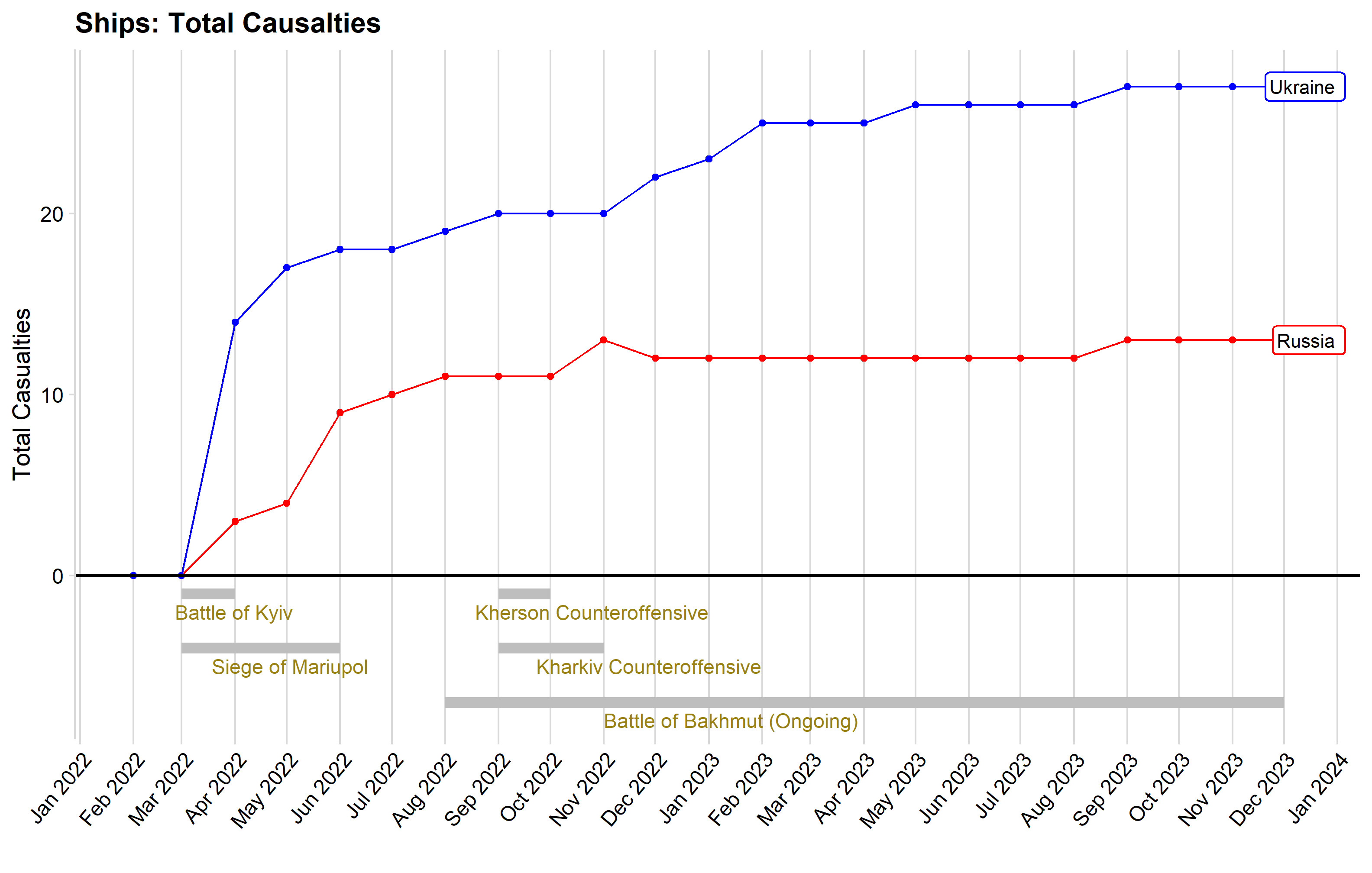
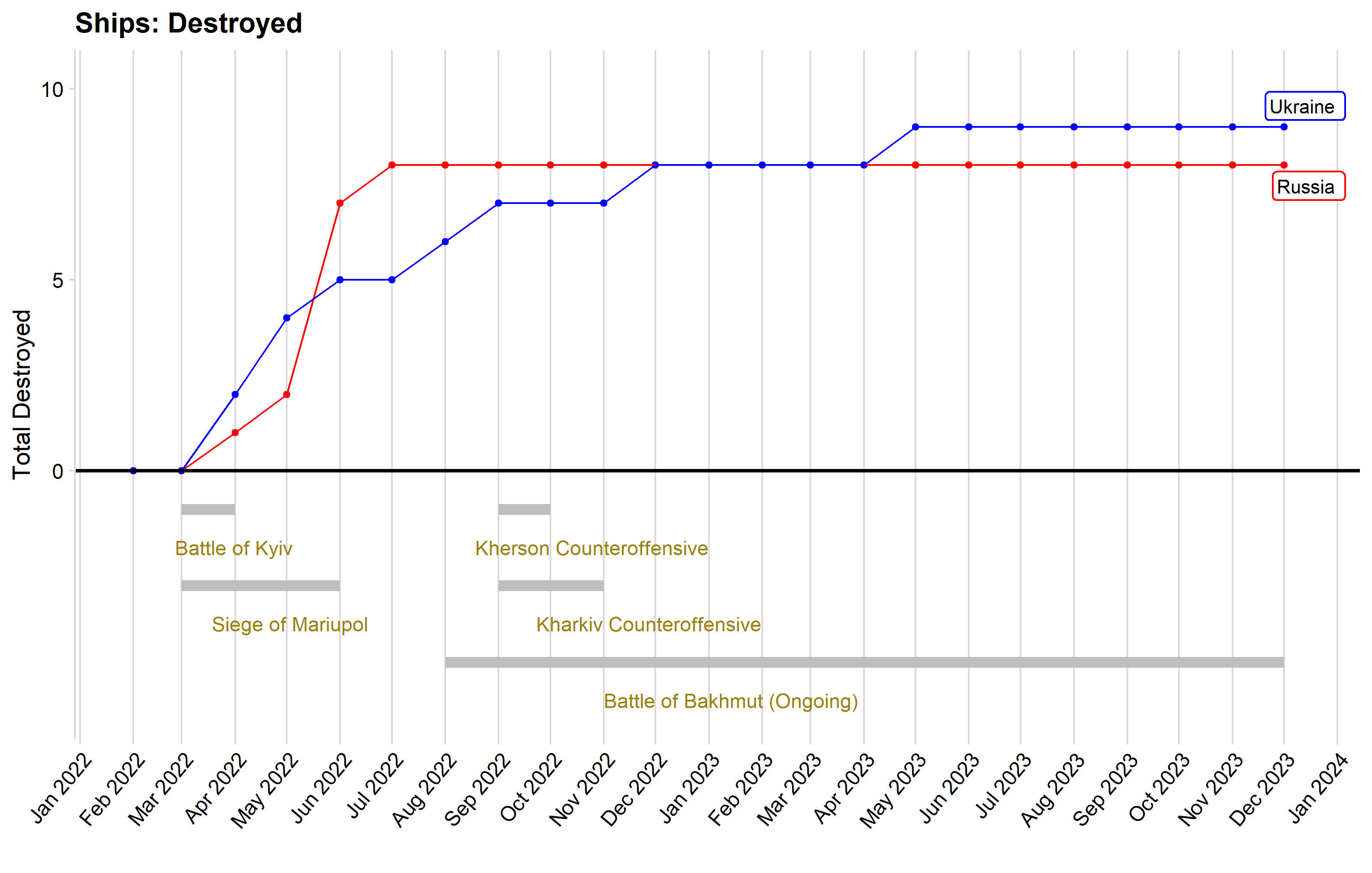
The below charts indicate that Russia has had an easier time of things when it comes to naval casualties. Ukraine has had consistent naval casualties throughout the war, while Russia has only lost 2 ships since September 2022.
Interestingly, the majority of Ukraine’s ship casualties have been ships captured by Russia. Ukraine have failed to capture any Russian ships. This helps to indicate that the vast majority of Ukraine’s resources are devoted to land power.
Of note is a spike in Russia’s casualties from 5/1/2022 to 6/1/2022. This follows the sinking of the Moskva, the Russian Black Sea flagship in April of 2022, which corresponds to the aid that was pledged during the beginning of the war.
ships_df <- ships %>%mutate(Date =fct_inorder(Date, TRUE) %>%mdy()) %>%complete(country,Date =seq(mdy("2/1/2022"), min(Date), by ="1 month"),fill =list(destroyed = 0L,damaged = 0L,captured = 0L,abandoned = 0L,type_total = 0L ) ) %>%complete(country, Date =seq(min(Date), max(Date), by ="1 month")) %>%mutate(equipment_type =replace_na(equipment_type, "Naval Ships") ) %>%group_by(country) %>%arrange(country, Date) %>%fill(destroyed, .direction ='down') %>%fill(abandoned, .direction ='down') %>%fill(damaged, .direction ='down') %>%fill(type_total, .direction ='down') %>%fill(captured, .direction ='down') %>%ungroup()ships_df %>%ggplot(aes(x = Date, y = type_total, color = country, group = country))+geom_point()+geom_line()+geom_segment(x=mdy("3/1/2022"), xend=mdy("4/1/2022"), y=-1, yend =-1, color ='grey', linewidth =3) +geom_segment(x=mdy("3/1/2022"), xend=mdy("6/1/2022"), y=-4, yend =-4, color ='grey', linewidth =3) +geom_segment(x=mdy("9/1/2022"), xend=mdy("11/1/2022"), y=-4, yend =-4, color ='grey', linewidth =3) +geom_segment(x=mdy("9/1/2022"), xend=mdy("10/1/2022"), y=-1, yend =-1, color ='grey', linewidth =3) +geom_segment(x=mdy("8/1/2022"), xend=mdy("12/1/2023"), y=-7, yend =-7, color ='grey', linewidth =3) +annotate(geom ='text', x =mdy("5/1/2022"), y =-2, hjust =0.95,label ='Battle of Kyiv', size =4, color ='#998114') +annotate(geom ='text', x =mdy("4/1/2022"), y =-5, hjust =0.15,label ='Siege of Mariupol', size =4, color ='#998114') +annotate(geom ='text', x =mdy("9/1/2022"), y =-2, hjust =0.1,label ='Kherson Counteroffensive', size =4, color ='#998114') +annotate(geom ='text', x =mdy("11/1/2022"), y =-5, hjust =0.3,label ='Kharkiv Counteroffensive', size =4, color ='#998114') +annotate(geom ='text', x =mdy("11/1/2022"), y =-8, hjust =0,label ='Battle of Bakhmut (Ongoing)', size =4, color ='#998114') +geom_hline(aes(yintercept =0), color ='black', size =1) +geom_label_repel(data =filter(ships_df, Date ==mdy("12/1/2023")), aes(color = country, label = country), hjust =-0,nudge_x =10, direction ="y", label.size =1,segment.color =NA ) +scale_color_manual(values =c("Russia"="red", "Ukraine"="blue")) +geom_label_repel(data =filter(ships_df, Date ==mdy("12/1/2023")), aes(label = country), color ="black", hjust =-0,nudge_x =10, direction ="y", label.size =NA,segment.color =NA ) +scale_x_date(date_labels ="%b %Y", date_breaks ="1 month", guide =guide_axis(angle =50))+scale_y_continuous(breaks =seq(min(ships_df$type_total), round(max(ships_df$type_total), digits =-1), by =10),expand =expansion(add =c(1, 2)) ) +labs(x ="", y ="Total Casualties", title ="Ships: Total Causalties")+theme_minimal_vgrid()+theme(legend.position ='none')
Code
ships_df <- ships %>%mutate(Date =fct_inorder(Date, TRUE) %>%mdy()) %>%complete(country,Date =seq(mdy("2/1/2022"), min(Date), by ="1 month"),fill =list(destroyed = 0L,damaged = 0L,captured = 0L,abandoned = 0L,type_total = 0L ) ) %>%complete(country, Date =seq(min(Date), max(Date), by ="1 month")) %>%mutate(equipment_type =replace_na(equipment_type, "Naval Ships") ) %>%group_by(country) %>%arrange(country, Date) %>%fill(destroyed, .direction ='down') %>%fill(abandoned, .direction ='down') %>%fill(damaged, .direction ='down') %>%fill(type_total, .direction ='down') %>%fill(captured, .direction ='down') %>%ungroup()ships_df %>%ggplot(aes(x = Date, y = destroyed, color = country, group = country))+geom_point()+geom_line()+geom_segment(x=mdy("3/1/2022"), xend=mdy("4/1/2022"), y=-1, yend =-1, color ='grey', linewidth =3) +geom_segment(x=mdy("3/1/2022"), xend=mdy("6/1/2022"), y=-3, yend =-3, color ='grey', linewidth =3) +geom_segment(x=mdy("9/1/2022"), xend=mdy("11/1/2022"), y=-3, yend =-3, color ='grey', linewidth =3) +geom_segment(x=mdy("9/1/2022"), xend=mdy("10/1/2022"), y=-1, yend =-1, color ='grey', linewidth =3) +geom_segment(x=mdy("8/1/2022"), xend=mdy("12/1/2023"), y=-5, yend =-5, color ='grey', linewidth =3) +annotate(geom ='text', x =mdy("5/1/2022"), y =-2, hjust =0.95,label ='Battle of Kyiv', size =4, color ='#998114') +annotate(geom ='text', x =mdy("4/1/2022"), y =-4, hjust =0.15,label ='Siege of Mariupol', size =4, color ='#998114') +annotate(geom ='text', x =mdy("9/1/2022"), y =-2, hjust =0.1,label ='Kherson Counteroffensive', size =4, color ='#998114') +annotate(geom ='text', x =mdy("11/1/2022"), y =-4, hjust =0.3,label ='Kharkiv Counteroffensive', size =4, color ='#998114') +annotate(geom ='text', x =mdy("11/1/2022"), y =-6, hjust =0,label ='Battle of Bakhmut (Ongoing)', size =4, color ='#998114') +geom_hline(aes(yintercept =0), color ='black', size =1) +geom_label_repel(data =filter(ships_df, Date ==mdy("12/1/2023")), aes(color = country, label = country), hjust =-0,nudge_x =10, direction ="y", label.size =1,segment.color =NA ) +scale_color_manual(values =c("Russia"="red", "Ukraine"="blue")) +geom_label_repel(data =filter(ships_df, Date ==mdy("12/1/2023")), aes(label = country), color ="black", hjust =-0,nudge_x =10, direction ="y", label.size =NA,segment.color =NA ) +scale_x_date(date_labels ="%b %Y", date_breaks ="1 month", guide =guide_axis(angle =50))+scale_y_continuous(breaks =seq(min(ships_df$destroyed), round(max(ships_df$destroyed), digits =-1), by =5),expand =expansion(add =c(1, 2)) ) +labs(x ="", y ="Total Destroyed", title ="Ships: Destroyed")+theme_minimal_vgrid()+theme(legend.position ='none')
Code
ships_df <- ships %>%mutate(Date =fct_inorder(Date, TRUE) %>%mdy()) %>%complete(country,Date =seq(mdy("2/1/2022"), min(Date), by ="1 month"),fill =list(destroyed = 0L,damaged = 0L,captured = 0L,abandoned = 0L,type_total = 0L ) ) %>%complete(country, Date =seq(min(Date), max(Date), by ="1 month")) %>%mutate(equipment_type =replace_na(equipment_type, "Naval Ships") ) %>%group_by(country) %>%arrange(country, Date) %>%fill(destroyed, .direction ='down') %>%fill(abandoned, .direction ='down') %>%fill(damaged, .direction ='down') %>%fill(type_total, .direction ='down') %>%fill(captured, .direction ='down') %>%ungroup()ships_df %>%ggplot(aes(x = Date, y = captured, color = country, group = country))+geom_point()+geom_line()+geom_segment(x=mdy("3/1/2022"), xend=mdy("4/1/2022"), y=-1, yend =-1, color ='grey', linewidth =3) +geom_segment(x=mdy("3/1/2022"), xend=mdy("6/1/2022"), y=-4, yend =-4, color ='grey', linewidth =3) +geom_segment(x=mdy("9/1/2022"), xend=mdy("11/1/2022"), y=-4, yend =-4, color ='grey', linewidth =3) +geom_segment(x=mdy("9/1/2022"), xend=mdy("10/1/2022"), y=-1, yend =-1, color ='grey', linewidth =3) +geom_segment(x=mdy("8/1/2022"), xend=mdy("12/1/2023"), y=-7, yend =-7, color ='grey', linewidth =3) +annotate(geom ='text', x =mdy("5/1/2022"), y =-2, hjust =0.95,label ='Battle of Kyiv', size =4, color ='#998114') +annotate(geom ='text', x =mdy("4/1/2022"), y =-5, hjust =0.15,label ='Siege of Mariupol', size =4, color ='#998114') +annotate(geom ='text', x =mdy("9/1/2022"), y =-2, hjust =0.1,label ='Kherson Counteroffensive', size =4, color ='#998114') +annotate(geom ='text', x =mdy("11/1/2022"), y =-5, hjust =0.3,label ='Kharkiv Counteroffensive', size =4, color ='#998114') +annotate(geom ='text', x =mdy("11/1/2022"), y =-8, hjust =0,label ='Battle of Bakhmut (Ongoing)', size =4, color ='#998114') +geom_hline(aes(yintercept =0), color ='black', size =1) +geom_label_repel(data =filter(ships_df, Date ==mdy("12/1/2023")), aes(color = country, label = country), hjust =-0,nudge_x =10, direction ="y", label.size =1,segment.color =NA ) +scale_color_manual(values =c("Russia"="red", "Ukraine"="blue")) +geom_label_repel(data =filter(ships_df, Date ==mdy("12/1/2023")), aes(label = country), color ="black", hjust =-0,nudge_x =10, direction ="y", label.size =NA,segment.color =NA ) +scale_x_date(date_labels ="%b %Y", date_breaks ="1 month", guide =guide_axis(angle =50))+scale_y_continuous(breaks =seq(min(ships_df$captured), max(ships_df$captured), by =5)) +labs(x ="", y ="Total Captured", title ="Ships: Captured")+theme_minimal_vgrid()+theme(legend.position ='none')
Conclusion
Our analysis of the casualties sustained by military personnel, tanks, aircraft, helicopters, and ships during the Russian invasion of Ukraine has yielded clear visualizations on the complexities of this conflict. The notable disparity in tank casualties presents a few options: either Ukrainian armored tactics and strategy is significantly superior to their Russian counterparts, Ukraine simply has fewer tanks to lose, or a combination of the two. The patterns in aircraft and helicopter casualties indicate a heated and complex aerial battle, with Ukraine gaining a slight edge, although the rates for both sides have been almost identical for the last year. Significantly, the increase in helicopter casualties for Russia aligns with the documented success of Ukrainian forces armed with sophisticated equipment, such as U.S. made MGM-140 ATACMS (Army M39) ballistic missiles, acquired through international aid.
Furthermore, our research highlights the influence of assistance in obtaining rather than the destruction of Russian tanks, indicating the implementation of subtle tactics by Ukraine. In order to enhance our comprehension, future research should thoroughly investigate the distinct categories and sources of aid, examining how these resources impact military tactics and results.
ALL MEMBERS CONTRIBITED EQUALLY
Data Dictionary
aid_col
Variable
Datatype
Description
X.1
integer
Miscellaneous index
X
integer
Miscellaneous index
Countries
character
Name of country
Announcement Date
character
Date of public announcement
Type.Of.Aid.General
character
Class of aid
Total
character
Total value in native currency
Converted.Value.in.EUR
character
Total value in Euros
Total_in_USD
double
Total value in US dollars
Date
character
Redundant of Announcement Date
Week
character
Date of start of current week
Month
character
Date of start of current month
Total_by_Country
double
Total contributed by country
Cumulative
douhble
Cumulative total inclusive
monthly_total
double
Total for the current month
total_aid_bar
Variable
Datatype
Description
X
integer
Miscellaneous index
Countries
character
Name of country
Total_by_Country
double
Total contributed by country
top_aid_months
Variable
Datatype
Description
X
integer
Miscellaneous index
Countries
character
Name of country
Announcement Date
character
Date of public announcement
Type.Of.Aid.General
character
Class of aid
Total
character
Total value in native currency
Converted.Value.in.EUR
character
Total value in Euros
Total_in_USD
double
Total value in US dollars
Date
character
Redundant of Announcement Date
Week
character
Date of start of current week
Month
character
Date of start of current month
Total_by_Country
double
Total contributed by country
equipment
Variable
Datatype
Description
X
integer
Miscellaneous index
country
character
Name of country
equipment_type
character
Type of equipment piece
destroyed
integer
Number of equipment pieces destroyed
abandoned
integer
Number of equipment pieces abandoned
captured
integer
Number of equipment pieces captured
damaged
integer
Number of equipment pieces damaged
type_total
integer
Total pieces of equipment casualties
Date
character
Date of record
tanks
Variable
Datatype
Description
X.1
integer
Miscellaneous index
X
integer
Miscellaneous index
country
character
Name of country
equipment_type
character
Type of equipment piece
destroyed
integer
Number of equipment pieces destroyed
abandoned
integer
Number of equipment pieces abandoned
captured
integer
Number of equipment pieces captured
damaged
integer
Number of equipment pieces damaged
type_total
integer
Total pieces of equipment casualties
Date
character
Date of record
aircraft
Variable
Datatype
Description
X.1
integer
Miscellaneous index
X
integer
Miscellaneous index
country
character
Name of country
equipment_type
character
Type of equipment piece
destroyed
integer
Number of equipment pieces destroyed
abandoned
integer
Number of equipment pieces abandoned
captured
integer
Number of equipment pieces captured
damaged
integer
Number of equipment pieces damaged
type_total
integer
Total pieces of equipment casualties
Date
character
Date of record
helicopters
Variable
Datatype
Description
X.1
integer
Miscellaneous index
X
integer
Miscellaneous index
country
character
Name of country
equipment_type
character
Type of equipment piece
destroyed
integer
Number of equipment pieces destroyed
abandoned
integer
Number of equipment pieces abandoned
captured
integer
Number of equipment pieces captured
damaged
integer
Number of equipment pieces damaged
type_total
integer
Total pieces of equipment casualties
Date
character
Date of record
ships
Variable
Datatype
Description
X.1
integer
Miscellaneous index
X
integer
Miscellaneous index
country
character
Name of country
equipment_type
character
Type of equipment piece
destroyed
integer
Number of equipment pieces destroyed
abandoned
integer
Number of equipment pieces abandoned
captured
integer
Number of equipment pieces captured
damaged
integer
Number of equipment pieces damaged
type_total
integer
Total pieces of equipment casualties
Date
character
Date of record
russia_personnel
Variable
Datatype
Description
date
date
Date of record
day
double
Day of war
personnel
double
Number of personnel lost
personnel*
character
Not sure
POW
double
Number of personnel lost as POW
russia_equipment
Variable
Datatype
Description
date
date
Date of record
day
double
Day of war
aircraft
double
Number of aircraft available
helicopter
double
Number of helicopters available
tank
double
Number of tanks available
APC
double
Number of APCs available
field artillery
double
Number of field artillery pieces available
MRL
double
Number of Multiple Rocket Launcers available
military auto
double
Number of military vehicles available
fuel tank
double
Number of aircraft available
aircraft
double
Number of aircraft available
aircraft
double
Number of aircraft available
aircraft
double
Number of aircraft available
aircraft
double
Number of aircraft available
personnel
double
Number of personnel lost
personnel*
character
Not sure
POW
double
Number of personnel lost as POW
Source Code
---title: "Ukraine After 21 Months"subtitle: "How has the war in Ukraine gone for both sides so far?"author: "Bogdan Bunea, Ian Milko, Collin Schwab, and Rayyan Hussien"date: December 10, 2023format: html: toc: true toc-location: left code-fold: true code-tools: true code-annotations: select theme: sandstone---```{r}#| label: setup #| include: false# install.packages("ggsci")# Load libraries and settings herelibrary(here)library(gganimate)library(cowplot)library(tidyverse)library(viridis)library(ggrepel)library(gganimate)library(magick)library(plotly)library(lubridate)library(ggsci)library(scales)knitr::opts_chunk$set(warning =FALSE,message =FALSE,comment ="#>",fig.path ="figs/", # Folder where rendered plots are savedfig.width =11, # Default plot widthfig.height =7, # Default plot heightfig.retina =3# For better plot resolution)# Put any other "global" settings here, e.g. a ggplot theme:theme_set(theme_bw(base_size =20))# Write code below here to load any data used in projectequipment <-read.csv(here('data_processed', "FullEquipCas.csv"))tanks <-read.csv(here('data_processed', "tanks.csv"))aircraft <-read.csv(here('data_processed', "aircraft.csv"))helicopters <-read.csv(here('data_processed', "helicopters.csv"))ships <-read.csv(here('data_processed', "ships.csv"))aid_col <-read.csv(here('data_processed', 'aid_col.csv'))top_aid_months <-read.csv(here('data_processed', 'top_aid_by_months.csv'))total_aid_bar <-read.csv(here('data_processed', 'total_aid_bar.csv'))russia_personnel <-read_csv(here('data_raw', 'russia_losses_personnel.csv'))russia_equipment <-read_csv(here('data_raw', 'russia_losses_equipment.csv'))```# Research QuestionHow have casualties changed as the Russian Invasion of Ukraine has progressed, and how have those casualties been impacted by different battles and the introduction of foreign aid?::: {.column-body}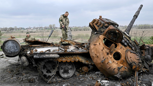{width=140%, height=140%}:::# IntroductionRussia sent shock waves around the world when they invaded Ukraine on the 24th of February, 2022. Russia being the military power that it is, many experts and journalists expected Ukraine to fold within a few months. However, this invasion was met not only with unprecedented determination by the people of Ukraine, but also with unprecedented military aid from around the world. The war has gone on and on, creating massive numbers of casualties as the fighting continues. This project aims to visualize and analyze Ukrainian and Russian casualties over the course of the war, and identify how foreign aid may have played a part during this war.# Data SourcesFor our research, data is split into two main categories: equipment and personnel losses, and total aid in dollar value donated by country. These two categories are crucial for visualizing what has been happening in Ukraine militarily for the last 21 months, while also creating a visual image of how aid shipments could have led to more carnage for Russian forces.Beginning with our aid datasets, we’ve used a plethora of different sources that all collaborate with each other while citing reputable sources. For example, the Ukraine Support Tracker is built off data from the Kiel Institute for the World Economy.When it comes to equipment and personnel losses, a different story takes place. As a result of the fog of war, as well as Russia refusing to release casualty numbers, all data are based off estimates and do not represent a complete and accurate count. That is why our data for personnel losses comes mainly from the General Staff of the Armed Forces of Ukraine. Equipment losses are a different story on the other hand, as one of our datasets verifies all major equipment losses (tanks, planes, helicopters, SAM sites, etc.) with geotagged images that corroborate these losses.Below is a more detailed breakdown of each dataset we used and the original link from which it was retrieved.#### US Weapons Export Dataset><https://www.kaggle.com/datasets/febinphilips/us-weapons-export-dataset>The above data set provides the USA's arms and weapons sales data to different countries from 1996 - 2022. The creator of the dataset does not list the their sources, making it somewhat suspect. However, different news sources do corroborate the data, so we are confident enough to use it.#### 2022 Russia Ukraine War><https://www.kaggle.com/datasets/piterfm/2022-ukraine-russian-war>The above dataset includes Russian equipment losses, personnel casualties, and prisoners of war (POWs) for 2022. This data was compiled from the Ukrainian Defence Ministry, Oryxspioenkop, and different interactive maps. Oryxpioenkop is a common source for statistics related to the war in Ukraine. It is important to remember that most, if not all, statistics regarding the war will be subject to propoganda by both sides and a fog of war that makes it nearly impossible to conclusively determine the accuracy of the data.#### IFW Kiel Ukraine Support Tracker<https://www.ifw-kiel.de/publications/ukraine-support-tracker-data-20758/>The above data is a listing of foreign aid sent to Ukraine. This is split between military, humanitarian, and financial aid. The source of this document is the Kiel Institute for the World Economy, which operates in part as an academic publisher. This information should be seen as trustworthy, as it is taken largely from each governments' statements on its own contributions. It should be taken with a slight grain of salt, however, as the donation of greater funds can be used propogandistically to make the donor country look better.# Presentation of Data## AidWe will begin by painting a picture of the foreign aid that was submitted so that readers will have an idea of the aid timeline when looking at plots later on. We first highlighted the top ten contributors of military aid to Ukraine, including the United States, Germany, the UK, and more. Our team then compiled the monthly output of aid from these top ten countries to show a timeline of when aid was introduced into the conflict. Readers will notice significant jumps in funding in the beginning of the war (February to April 2022), followed by a gradual rate until the new year, when we see another large jump. The lack of funding in the most recent months of the war may be because several countries choose to follow the US's lead. As American aid to Ukraine has slowed, so has aid from other countries, as illustrated in the third tab below. With the notable exception of the European Peace Facility, Norway, and Denmark, most countries' aid pledges have leveled off alongside the US. ::: {.panel-tabset}### Top Ten Aid Contributors```{r}total_aid_bar %>%slice(33,12,34,23,8,24,21,5,31,35) %>%mutate(Countries =fct_reorder(Countries, Total_by_Country)) %>%mutate(val_lbl =paste0(" ", round(Total_by_Country, digits =2))) %>%ggplot()+geom_col(aes(x = Total_by_Country, y = Countries)) +geom_text(aes(x = Total_by_Country, y = Countries, label = val_lbl, hjust =-0.2), size =4)+labs(x ="Total Military Aid (Billions of USD)", y ="", title ="Top Contributors of \nForeign Military Aid to Ukraine")+theme_minimal_vgrid()+theme(legend.position ='none',plot.margin =unit(c(0.5, 0.5, 0.5, 0), "cm"))+scale_x_continuous(expand =expansion(mult =c(0, 0.1)))```### Total Military Aid by Month```{r}aid_col %>%mutate(Month =fct_inorder(Month, TRUE) %>%mdy()) %>%mutate(val_lbl =paste0(" ", round(monthly_total, digits =2))) %>%ggplot()+geom_col(aes(x = Month, y = monthly_total))+geom_text(aes(x = Month, y = monthly_total, label = val_lbl, vjust =-1), size =3)+labs(x ="", y ="Total Military Aid (Billions of USD)", title ="Cumulative Military Aid by Month", subtitle ="From Top Ten Contributing Countries")+theme_minimal_hgrid()+scale_x_date(date_labels ="%b %Y", date_breaks ="1 month", guide =guide_axis(angle =50))```### Top Aid Contributors by Month```{r}tam_df <- top_aid_months %>%mutate(Month =fct_inorder(Month, TRUE) %>%mdy()) %>%mutate(Cumulative = Cumulative /10^9) %>%mutate(Countries =ifelse(Countries =="United Kingdom", "Rest of Top Ten", Countries))tam_df %>%ggplot(aes(x = Month, y = Cumulative, group = Countries))+geom_point(aes(color = Countries))+geom_line(aes(color = Countries))+geom_label_repel(data =filter(tam_df, (Month ==mdy("7/1/2023")) & (Countries %in%c("United States", "Germany", "Rest of Top Ten"))), aes(color = Countries, label = Countries), hjust =-0,nudge_x =10, direction ="y", label.size =1,segment.color =NA ) +scale_color_simpsons() +geom_label_repel(data =filter(tam_df, (Month ==mdy("7/1/2023")) & (Countries %in%c("United States", "Germany", "Rest of Top Ten"))), aes(label = Countries), color ="black", hjust =-0,nudge_x =10, direction ="y", label.size =NA,segment.color =NA ) +labs(x ="",y ="Aid Pledged (Billions of USD)",title ="Cumulative Monthly Aid Pledged to Ukraine",subtitle ="By Top Ten Contributing Countries/Organizations")+theme_minimal_grid()+theme(legend.position ='none') +scale_x_date(date_labels ="%b %Y", date_breaks ="1 month", guide =guide_axis(angle =50))``````{r}tam_df2 <- top_aid_months %>%filter(Countries !="United States") %>%filter(Countries !="Germany") %>%mutate(Month =fct_inorder(Month, TRUE) %>%mdy()) %>%mutate(Cumulative = Cumulative /10^9)tam_df2 %>%ggplot(aes(x = Month, y = Cumulative, group = Countries))+geom_point(aes(color = Countries))+geom_line(aes(color = Countries))+geom_label_repel(data =filter(tam_df2, Month ==mdy("7/1/2023")), aes(color = Countries, label = Countries), hjust =-0,nudge_x =10, direction ="y", label.size =1,segment.color =NA ) +scale_color_simpsons() +geom_label_repel(data =filter(tam_df2, Month ==mdy("7/1/2023")), aes(label = Countries), color ="black", hjust =-0,nudge_x =10, direction ="y", label.size =NA,segment.color =NA ) +labs(x ="",y ="Aid Pledged (Billions of USD)",title ="Cumulative Monthly Aid Pledged to Ukraine",subtitle ="Countries ranked 2 - 8")+scale_x_date(date_labels ="%b %Y", date_breaks ="1 month", guide =guide_axis(angle =50), expand =expansion(mult =c(0.05, 0.1))) +theme_minimal_grid() +theme(legend.position ='none')```:::## Military Losses::: {.panel-tabset}### Personnel LossesDisplayed in the chart below, a Ukrainian Military estimate of Russian Causalities over the course of the war is shown. With this chart, a clear escalation in casualties occurs especially after Week 17 of the war which is when the first major shipment of heavy weaponry was delivered from Germany. ```{r}weekly <- russia_personnel %>%select(-POW,-`personnel*`) %>%mutate(week =floor_date(date, unit ="week"),daily_losses =c(NA, diff(personnel)),daily_losses_shifted =lead(daily_losses)) %>%group_by(week) %>%mutate(week_label =cur_group_id()) %>%group_by(week_label) %>%summarise(week_total =sum(daily_losses_shifted) ) %>%mutate(fill_color =ifelse(week_total <mean(week_total, na.rm =TRUE), "red", "blue")) %>%mutate(count_before =sum(week_label <17& fill_color =="blue", na.rm =TRUE),count_after =sum(week_label >=17& fill_color =="blue", na.rm =TRUE) ) %>%mutate(Week_Number = week_label,Week_Total = week_total )graph2 <- weekly %>%ggplot() +geom_bar(aes(x = Week_Number, y = Week_Total, fill = fill_color), stat ="identity", width =1) +theme_cowplot() +scale_fill_manual(values =c("red"="grey50", "blue"="red3")) +scale_x_continuous(expand =expand_scale(mult =c(0.01, 0.1))) +scale_y_continuous(labels = comma,expand =expand_scale(mult =c(0.03, 0.1))) +labs(x ="Week Number",y ="Weekly Total",title ="Ukrainian Estimates of Russian Personnel Casualities",caption ="Data up to Nov/26/2023" ) +geom_segment(x=(1), xend=(6), y=-100, yend =-100, color ='grey', linewidth =1, alpha =0.1) +geom_segment(x=(1), xend=(15), y=-700, yend =-700, color ='grey', linewidth =1, alpha =0.1) +geom_segment(x=(27), xend=(31), y=-100, yend =-100, color ='grey', linewidth =1, alpha =0.1) +geom_segment(x=(27), xend=(34), y=-700, yend =-700, color ='grey', linewidth =1, alpha =0.1) +geom_segment(x=(24), xend=(93), y=-1300, yend =-1300, color ='grey', linewidth =1, alpha =0.1) +annotate(geom ='text', x =6, y =-350,label ='Battle of Kyiv', size =3, color ='black') +annotate(geom ='text', x =8, y =-1000,label ='Siege of Mariupol', size =3, color ='black') +annotate(geom ='text', x =37, y =-350,label ='Kherson Counteroffensive', size =3, color ='black') +annotate(geom ='text', x =39, y =-1000,label ='Kharkiv Counteroffensive', size =3, color ='black') +annotate(geom ='text', x =45, y =-1650,label ='Battle of Bakhmut (Ongoing)', size =3, color ='black') +theme(plot.title =element_text(hjust =0, size =12),legend.position ="none")+geom_text(data =data.frame(x =30.5, y =7175, label =paste("Count Exceeding Mean Before 17 Weeks: ",weekly$count_before)),mapping =aes(x = x, y = y, label = label),inherit.aes =FALSE) +geom_text(data =data.frame(x =30.5, y =6720, label =paste("Count Exceeding Mean After 17 Weeks: ",weekly$count_after)),mapping =aes(x = x, y = y, label = label),inherit.aes =FALSE) +geom_hline(yintercept =mean(weekly$week_total, na.rm =TRUE),linetype ='dashed' ) +annotate('text', x =18, y =3750,color ='black', hjust =1,label ='Mean Casuality Estimates')ggplotly( graph2,tooltip =c("Week_Number","Week_Total"))```### Equipment LossesThis chart illustrates the cumulative monthly summary of equipment loss for Russia and Ukraine from March 2022 to December 2023. The y-axis represents the total equipment loss values, encompassing various categories such as destroyed, abandoned, captured, and damaged pieces, while the x-axis denotes the timeline. The data provides crucial insights into the military dynamics of the conflict. Notably, the graph reveals a stark disparity in the impact on Russia’s and Ukraine’s equipment, with Russia experiencing significantly higher losses, particularly evident after the initial three months. After that period, Russia’s impacted equipment surpasses Ukraine’s by a considerable margin, reaching twice the number. This discrepancy sheds light on the differing degrees of resilience and adaptability demonstrated by the two nations in the face of the ongoing conflict.```{r}equip_summary_df <-read_csv(here("data_processed", "FilteredEquipSummaryByMonth.csv")) %>%mutate(Date =fct_inorder(Date, TRUE) %>%mdy()) %>%mutate(Country =str_to_title(Country))equip_summary_df %>%ggplot(aes(x = Date, y = Total_Values, color = Country, group = Country)) +geom_point() +geom_line() +geom_segment(x=mdy("3/1/2022"), xend=mdy("4/1/2022"), y=-1000, yend =-1000, color ='grey', linewidth =3) +geom_segment(x=mdy("3/1/2022"), xend=mdy("6/1/2022"), y=-2500, yend =-2500, color ='grey', linewidth =3) +geom_segment(x=mdy("9/1/2022"), xend=mdy("11/1/2022"), y=-2500, yend =-2500, color ='grey', linewidth =3) +geom_segment(x=mdy("9/1/2022"), xend=mdy("10/1/2022"), y=-1000, yend =-1000, color ='grey', linewidth =3) +geom_segment(x=mdy("8/1/2022"), xend=mdy("12/1/2023"), y=-4000, yend =-4000, color ='grey', linewidth =3) +annotate(geom ='text', x =mdy("6/1/2022"), y =-1500, hjust =1.6,label ='Battle of Kyiv', size =4, color ='#998114') +annotate(geom ='text', x =mdy("4/1/2022"), y =-3000, hjust =0.15,label ='Siege of Mariupol', size =4, color ='#998114') +annotate(geom ='text', x =mdy("9/1/2022"), y =-1500, hjust =0.4,label ='Kherson Counteroffensive', size =4, color ='#998114') +annotate(geom ='text', x =mdy("11/1/2022"), y =-3000, hjust =0.9,label ='Kharkiv Counteroffensive', size =4, color ='#998114') +annotate(geom ='text', x =mdy("12/1/2022"), y =-4500, hjust =-0.5,label ='Battle of Bakhmut (Ongoing)', size =4, color ='#998114') +geom_hline(aes(yintercept =0), color ='black', size =1) +geom_label_repel(data =filter(equip_summary_df, Date ==mdy("12/1/2023")), aes(color = Country, label = Country), hjust =-0,nudge_x =10, direction ="y", label.size =1,segment.color =NA ) +scale_color_manual(values =c("Russia"="red", "Ukraine"="blue")) +geom_label_repel(data =filter(equip_summary_df, Date ==mdy("12/1/2023")), aes(label = Country), color ="black", hjust =-0,nudge_x =10, direction ="y", label.size =NA,segment.color =NA ) +labs(x ="",y ="Total Lost (Number of individual pieces)",title ="Cumulative Monthly Summary of Equipment Loss",subtitle ="By Country",caption ="" ) +scale_y_continuous(breaks =seq(round(min(equip_summary_df$Total_Values), digits =-3), round(max(equip_summary_df$Total_Values) +2000, digits =-3), by =2000),labels = comma,expand =expand_scale(mult =c(0.1, 0.1)) ) +scale_x_date(date_labels ="%b %Y", date_breaks ="1 month", guide =guide_axis(angle =50)) +theme_minimal_vgrid() +theme(legend.position ='none')```:::## TanksThe below charts show the differences between Russian and Ukrainian tank casualties over the course of the war. The first four charts show cumulative losses. The majority of tank casualties are from destroyed tanks, but Russia has also had many of their tanks either captured or abandoned. There is a rather sharp slope to Russia's casualties at the beginning of the war, corresponding with not only the Battle of Kyiv and Siege of Mariupol, but also with the large amounts of aid that were pledged within the first few months of the war. There was also a huge increase of captured Russian tanks from 9/1/2022 through 11/1/2022. This corresponds with a plateau in aid from the international community. This may indicate that Ukraine was trying to capture tanks for their own use instead of destroying them due to their lack of purchasing power/inventory. Alternatively, it may be because of the Russian's over extension into Ukraine and the lack of supply lines needed for refueling during the Kharkiv and Kherson Counteroffensives. As you can see in the final tab "Confirmed Tank Casualties", the chart compares the data to the mean to determine if a certain week exceeded the mean or not. This count starts at week 17 of the war as this is when the first notable heavy military equipment has been delierved to Ukraine.It should be noted that while there was a steep increase in aid at the beginning of 2023, the slope of both countries casualties stayed relatively constant. This indicates that either funding to the Ukraine was needed just to keep pace with Russia, or the aid was being used in other forms of combat.::: {.panel-tabset}### Total Tank Casualties```{r}tanks_df <- tanks %>%mutate(Date =fct_inorder(Date, TRUE) %>%mdy())tanks_df %>%ggplot(aes(x = Date, y = type_total, color = country, group = country))+geom_point()+geom_line()+geom_segment(x=mdy("3/1/2022"), xend=mdy("4/1/2022"), y=-100, yend =-100, color ='grey', linewidth =3) +geom_segment(x=mdy("3/1/2022"), xend=mdy("6/1/2022"), y=-350, yend =-350, color ='grey', linewidth =3) +geom_segment(x=mdy("9/1/2022"), xend=mdy("11/1/2022"), y=-350, yend =-350, color ='grey', linewidth =3) +geom_segment(x=mdy("9/1/2022"), xend=mdy("10/1/2022"), y=-100, yend =-100, color ='grey', linewidth =3) +geom_segment(x=mdy("8/1/2022"), xend=mdy("12/1/2023"), y=-600, yend =-600, color ='grey', linewidth =3) +annotate(geom ='text', x =mdy("5/1/2022"), y =-200, hjust =0.95,label ='Battle of Kyiv', size =4, color ='#998114') +annotate(geom ='text', x =mdy("4/1/2022"), y =-450, hjust =0.2,label ='Siege of Mariupol', size =4, color ='#998114') +annotate(geom ='text', x =mdy("9/1/2022"), y =-200, hjust =0.1,label ='Kherson Counteroffensive', size =4, color ='#998114') +annotate(geom ='text', x =mdy("11/1/2022"), y =-450, hjust =0.6,label ='Kharkiv Counteroffensive', size =4, color ='#998114') +annotate(geom ='text', x =mdy("11/1/2022"), y =-700, hjust =-0.5,label ='Battle of Bakhmut (Ongoing)', size =4, color ='#998114') +geom_hline(aes(yintercept =0), color ='black', size =1) +geom_label_repel(data =filter(tanks_df, Date ==mdy("12/1/2023")), aes(color = country, label = country), hjust =-0,nudge_x =10, direction ="y", label.size =1,segment.color =NA ) +scale_color_manual(values =c("Russia"="red", "Ukraine"="blue")) +geom_label_repel(data =filter(tanks_df, Date ==mdy("12/1/2023")), aes(label = country), color ="black", hjust =-0,nudge_x =10, direction ="y", label.size =NA,segment.color =NA ) +labs(x ="", y ="Total Casualties", title ="Tanks: Total Causalties") +scale_x_date(guide =guide_axis(angle =50), date_labels ="%b %Y", date_breaks ="1 month") +scale_y_continuous(breaks =seq(round(min(tanks_df$type_total), digits =-2), round(max(tanks_df$type_total), digits =-2), by =500),labels = comma,expand =expansion(mult =c(0.03, 0.05)) ) +theme_minimal_vgrid()+theme(legend.position ='none')```### Destroyed Tanks```{r}tanks_df <- tanks %>%mutate(Date =fct_inorder(Date, TRUE) %>%mdy())tanks_df %>%ggplot(aes(x = Date, y = destroyed, color = country, group = country))+geom_point()+geom_line()+geom_segment(x=mdy("3/1/2022"), xend=mdy("4/1/2022"), y=-100, yend =-100, color ='grey', linewidth =3) +geom_segment(x=mdy("3/1/2022"), xend=mdy("6/1/2022"), y=-350, yend =-350, color ='grey', linewidth =3) +geom_segment(x=mdy("9/1/2022"), xend=mdy("11/1/2022"), y=-350, yend =-350, color ='grey', linewidth =3) +geom_segment(x=mdy("9/1/2022"), xend=mdy("10/1/2022"), y=-100, yend =-100, color ='grey', linewidth =3) +geom_segment(x=mdy("8/1/2022"), xend=mdy("12/1/2023"), y=-600, yend =-600, color ='grey', linewidth =3) +annotate(geom ='text', x =mdy("5/1/2022"), y =-200, hjust =0.95,label ='Battle of Kyiv', size =4, color ='#998114') +annotate(geom ='text', x =mdy("4/1/2022"), y =-450, hjust =0.15,label ='Siege of Mariupol', size =4, color ='#998114') +annotate(geom ='text', x =mdy("9/1/2022"), y =-200, hjust =0.1,label ='Kherson Counteroffensive', size =4, color ='#998114') +annotate(geom ='text', x =mdy("11/1/2022"), y =-450, hjust =0.3,label ='Kharkiv Counteroffensive', size =4, color ='#998114') +annotate(geom ='text', x =mdy("11/1/2022"), y =-700, hjust =0,label ='Battle of Bakhmut (Ongoing)', size =4, color ='#998114') +geom_hline(aes(yintercept =0), color ='black', size =1) +geom_label_repel(data =filter(tanks_df, Date ==mdy("12/1/2023")), aes(color = country, label = country), hjust =-0,nudge_x =10, direction ="y", label.size =1,segment.color =NA ) +scale_color_manual(values =c("Russia"="red", "Ukraine"="blue")) +geom_label_repel(data =filter(tanks_df, Date ==mdy("12/1/2023")), aes(label = country), color ="black", hjust =-0,nudge_x =10, direction ="y", label.size =NA,segment.color =NA ) +labs(x ="", y ="Tanks Destroyed", title ="Tanks: Destroyed")+scale_x_date(guide =guide_axis(angle =50), date_labels ="%b %Y", date_breaks ="1 month") +scale_y_continuous(breaks =seq(round(min(tanks_df$destroyed), digits =-2), round(max(tanks_df$destroyed), digits =-2), by =500),labels = comma,expand =expansion(mult =c(0.03, 0.05)) ) +theme_minimal_vgrid()+theme(legend.position ='none')```### Captured Tanks```{r}tanks_df <- tanks %>%mutate(Date =fct_inorder(Date, TRUE) %>%mdy())tanks_df %>%ggplot(aes(x = Date, y = captured, color = country, group = country))+geom_point()+geom_line()+geom_segment(x=mdy("3/1/2022"), xend=mdy("4/1/2022"), y=-50, yend =-50, color ='grey', linewidth =3) +geom_segment(x=mdy("3/1/2022"), xend=mdy("6/1/2022"), y=-150, yend =-150, color ='grey', linewidth =3) +geom_segment(x=mdy("9/1/2022"), xend=mdy("11/1/2022"), y=-150, yend =-150, color ='grey', linewidth =3) +geom_segment(x=mdy("9/1/2022"), xend=mdy("10/1/2022"), y=-50, yend =-50, color ='grey', linewidth =3) +geom_segment(x=mdy("8/1/2022"), xend=mdy("12/1/2023"), y=-250, yend =-250, color ='grey', linewidth =3) +annotate(geom ='text', x =mdy("5/1/2022"), y =-100, hjust =0.95,label ='Battle of Kyiv', size =4, color ='#998114') +annotate(geom ='text', x =mdy("4/1/2022"), y =-200, hjust =0.15,label ='Siege of Mariupol', size =4, color ='#998114') +annotate(geom ='text', x =mdy("9/1/2022"), y =-100, hjust =0.1,label ='Kherson Counteroffensive', size =4, color ='#998114') +annotate(geom ='text', x =mdy("11/1/2022"), y =-200, hjust =0.3,label ='Kharkiv Counteroffensive', size =4, color ='#998114') +annotate(geom ='text', x =mdy("11/1/2022"), y =-300, hjust =0,label ='Battle of Bakhmut (Ongoing)', size =4, color ='#998114') +geom_hline(aes(yintercept =0), color ='black', size =1) +geom_label_repel(data =filter(tanks_df, Date ==mdy("12/1/2023")), aes(color = country, label = country), hjust =-0,nudge_x =10, direction ="y", label.size =1,segment.color =NA ) +scale_color_manual(values =c("Russia"="red", "Ukraine"="blue")) +scale_y_continuous(labels =c(0,500), breaks =c(0,500))+geom_label_repel(data =filter(tanks_df, Date ==mdy("12/1/2023")), aes(label = country), color ="black", hjust =-0,nudge_x =10, direction ="y", label.size =NA,segment.color =NA ) +labs(x ="", y ="Tanks Captured", title ="Tanks: Captured")+scale_x_date(guide =guide_axis(angle =50), date_labels ="%b %Y", date_breaks ="1 month") +scale_y_continuous(breaks =seq(round(min(tanks_df$captured), digits =-2), round(max(tanks_df$captured), digits =-2), by =200),labels = comma,expand =expansion(mult =c(0.03, 0.1)) ) +theme_minimal_vgrid()+theme(legend.position ='none')```### Abandoned Tanks```{r}tanks_df <- tanks %>%mutate(Date =fct_inorder(Date, TRUE) %>%mdy())tanks_df %>%ggplot(aes(x = Date, y = abandoned, color = country, group = country))+geom_point()+geom_line()+geom_segment(x=mdy("3/1/2022"), xend=mdy("4/1/2022"), y=-20, yend =-20, color ='grey', linewidth =3) +geom_segment(x=mdy("3/1/2022"), xend=mdy("6/1/2022"), y=-40, yend =-40, color ='grey', linewidth =3) +geom_segment(x=mdy("9/1/2022"), xend=mdy("11/1/2022"), y=-40, yend =-40, color ='grey', linewidth =3) +geom_segment(x=mdy("9/1/2022"), xend=mdy("10/1/2022"), y=-20, yend =-20, color ='grey', linewidth =3) +geom_segment(x=mdy("8/1/2022"), xend=mdy("12/1/2023"), y=-60, yend =-60, color ='grey', linewidth =3) +annotate(geom ='text', x =mdy("5/1/2022"), y =-30, hjust =0.95,label ='Battle of Kyiv', size =4, color ='#998114') +annotate(geom ='text', x =mdy("4/1/2022"), y =-50, hjust =0.15,label ='Siege of Mariupol', size =4, color ='#998114') +annotate(geom ='text', x =mdy("9/1/2022"), y =-30, hjust =0.1,label ='Kherson Counteroffensive', size =4, color ='#998114') +annotate(geom ='text', x =mdy("11/1/2022"), y =-50, hjust =0.3,label ='Kharkiv Counteroffensive', size =4, color ='#998114') +annotate(geom ='text', x =mdy("11/1/2022"), y =-70, hjust =0,label ='Battle of Bakhmut (Ongoing)', size =4, color ='#998114') +geom_hline(aes(yintercept =0), color ='black', size =1) +geom_label_repel(data =filter(tanks_df, Date ==mdy("12/1/2023")), aes(color = country, label = country), hjust =-0,nudge_x =10, direction ="y", label.size =1,segment.color =NA ) +scale_color_manual(values =c("Russia"="red", "Ukraine"="blue")) +geom_label_repel(data =filter(tanks_df, Date ==mdy("12/1/2023")), aes(label = country), color ="black", hjust =-0,nudge_x =10, direction ="y", label.size =NA,segment.color =NA ) +labs(x ="", y ="Tanks Abandoned", title ="Tanks: Abandoned")+scale_x_date(date_labels ="%b %Y", date_breaks ="1 month", guide =guide_axis(angle =50)) +scale_y_continuous(breaks =seq(round(min(tanks_df$abandoned), digits =-2), round(max(tanks_df$abandoned), digits =-2), by =50),labels = comma,expand =expansion(mult =c(0.03, 0.1)) ) +theme_minimal_vgrid()+theme(legend.position ='none')```### Confirmed Tank Casualities```{r}weekly_tank <- russia_equipment %>%select(date,day,tank) %>%mutate(week =floor_date(date, unit ="week"),daily_losses =c(NA, diff(tank)),daily_losses_shifted =lead(daily_losses)) %>%group_by(week) %>%mutate(week_label =cur_group_id()) %>%group_by(week_label) %>%summarise(week_total =sum(daily_losses_shifted) ) %>%mutate(fill_color =ifelse(week_total <mean(week_total, na.rm =TRUE), "red", "blue")) %>%mutate(count_before =sum(week_label <17& fill_color =="blue", na.rm =TRUE),count_after =sum(week_label >=17& fill_color =="blue", na.rm =TRUE)) %>%mutate(Week_Number = week_label,Week_Total = week_total )graph1 <- weekly_tank %>%ggplot() +geom_bar(aes(x = Week_Number, y = Week_Total, fill = fill_color), stat ="identity", width =1) +theme_cowplot() +scale_fill_manual(values =c("red"="grey50", "blue"="red3")) +scale_x_continuous(expand =expand_scale(mult =c(0.01, 0.1))) +scale_y_continuous(labels = comma,expand =expand_scale(mult =c(0.03, 0.1))) +labs(x ="Week Number",y ="Weekly Total",title ="Confirmed Russian Tank Casualities",caption ="Data up to Nov/26/2023" ) +geom_segment(x=(1), xend=(6), y=-5, yend =-5, color ='grey', linewidth =1, alpha =0.1) +geom_segment(x=(1), xend=(15), y=-16, yend =-16, color ='grey', linewidth =1, alpha =0.1) +geom_segment(x=(27), xend=(31), y=-5, yend =-5, color ='grey', linewidth =1, alpha =0.1) +geom_segment(x=(27), xend=(34), y=-16, yend =-16, color ='grey', linewidth =1, alpha =0.1) +geom_segment(x=(24), xend=(93), y=-27, yend =-27, color ='grey', linewidth =1, alpha =0.1) +annotate(geom ='text', x =6, y =-11,label ='Battle of Kyiv', size =3, color ='black') +annotate(geom ='text', x =8, y =-22,label ='Siege of Mariupol', size =3, color ='black') +annotate(geom ='text', x =37, y =-10,label ='Kherson Counteroffensive', size =3, color ='black') +annotate(geom ='text', x =39, y =-22,label ='Kharkiv Counteroffensive', size =3, color ='black') +annotate(geom ='text', x =45, y =-33,label ='Battle of Bakhmut (Ongoing)', size =3, color ='black') +geom_hline(aes(yintercept =0), color ='black', size =1) +theme(plot.title =element_text(hjust =0),legend.position ="none") +geom_text(data =data.frame(x =60, y =160, label =paste("Count Exceeding Mean Before 17 Weeks: ",weekly_tank$count_before)),mapping =aes(x = x, y = y, label = label),inherit.aes =FALSE) +geom_text(data =data.frame(x =60, y =150, label =paste("Count Exceeding Mean After 17 Weeks: ",weekly_tank$count_after)),mapping =aes(x = x, y = y, label = label),inherit.aes =FALSE, ) +geom_hline(yintercept =mean(weekly_tank$week_total, na.rm =TRUE),color ='black',linetype ='dashed' ) +annotate('text', x =45, y =59,color ='black', hjust =1,label ='Mean Tank\n Casualities',size =3)ggplotly(graph1 ,tooltip =c("Week_Number","Week_Total")) ```:::## Aircraft The following graphs illustrate the difference between cumulative Russian and Ukrainian aircraft casualties. The non-helicopter plots show a much closer war than the tank plots. In fact, our team would make the assumption that Russia is winning the aerial battle in terms of percentage of aircraft fleets lost, but we do not have access to the inventory of either country's fleets at the beginning of the invasion.Russia faced huge helicopter casualties in the first 2 months of the war. Nearly 33% of their helicopter casualties occurred during these months. Again, this corresponds to the huge amounts of aid that were pledged in the first months, as well as the Battle of Kyiv and Siege of Mariupol. Russia also faced a steep increase in helicopter casualties during October this year. Unfortunately, our aid data set only goes through July this year, so we cannot attribute these casualties directly to aid. However, we can infer from news sources that Ukrainian troops have become more and more effective with their donated weapon systems, to include the US-made Patriot missile system. This would account for the dramatic increase of destroyed Russian helicopters.These graphs illustrate a quick start to the war in terms of aircraft casualties, corresponding with aid pledges and the Battle of Kyiv and the Siege of Mariupol. Non-helicopter aircraft casualties have been relatively consistent month over month since 9/1/2022, but helicopter casualties for Russia continue to grow at an alarming rate.::: {.panel-tabset}### Total Aircraft Casualties```{r}aircraft_df <- aircraft %>%mutate(Date =fct_inorder(Date, TRUE) %>%mdy())aircraft_df %>%ggplot(aes(x = Date, y = type_total, color = country, group = country))+geom_point()+geom_line()+geom_segment(x=mdy("3/1/2022"), xend=mdy("4/1/2022"), y=-10, yend =-10, color ='grey', linewidth =3) +geom_segment(x=mdy("3/1/2022"), xend=mdy("6/1/2022"), y=-25, yend =-25, color ='grey', linewidth =3) +geom_segment(x=mdy("9/1/2022"), xend=mdy("11/1/2022"), y=-25, yend =-25, color ='grey', linewidth =3) +geom_segment(x=mdy("9/1/2022"), xend=mdy("10/1/2022"), y=-10, yend =-10, color ='grey', linewidth =3) +geom_segment(x=mdy("8/1/2022"), xend=mdy("12/1/2023"), y=-40, yend =-40, color ='grey', linewidth =3) +annotate(geom ='text', x =mdy("5/1/2022"), y =-15, hjust =0.95,label ='Battle of Kyiv', size =4, color ='#998114') +annotate(geom ='text', x =mdy("4/1/2022"), y =-30, hjust =0.15,label ='Siege of Mariupol', size =4, color ='#998114') +annotate(geom ='text', x =mdy("9/1/2022"), y =-15, hjust =0.1,label ='Kherson Counteroffensive', size =4, color ='#998114') +annotate(geom ='text', x =mdy("11/1/2022"), y =-30, hjust =0.3,label ='Kharkiv Counteroffensive', size =4, color ='#998114') +annotate(geom ='text', x =mdy("11/1/2022"), y =-45, hjust =0,label ='Battle of Bakhmut (Ongoing)', size =4, color ='#998114') +geom_hline(aes(yintercept =0), color ='black', size =1) +geom_label_repel(data =filter(aircraft_df, Date ==mdy("12/1/2023")), aes(color = country, label = country), hjust =-0,nudge_x =10, direction ="y", label.size =1,segment.color =NA ) +scale_color_manual(values =c("Russia"="red", "Ukraine"="blue")) +geom_label_repel(data =filter(aircraft_df, Date ==mdy("12/1/2023")), aes(label = country), color ="black", hjust =-0,nudge_x =10, direction ="y", label.size =NA,segment.color =NA ) +labs(x ="", y ="Aircraft Casualties", title ="Aircraft: Total Causalties")+scale_x_date(date_labels ="%b %Y", date_breaks ="1 month", guide =guide_axis(angle =50)) +scale_y_continuous(breaks =seq(round(min(aircraft_df$type_total), digits =-1), round(max(aircraft_df$type_total), digits =-2), by =20),expand =expansion(mult =c(0.03, 0.05)) ) +theme_minimal_vgrid()+theme(legend.position ='none')```### Destroyed Aircraft```{r}aircraft_df <- aircraft %>%mutate(Date =fct_inorder(Date, TRUE) %>%mdy())aircraft_df %>%ggplot(aes(x = Date, y = destroyed, color = country, group = country))+geom_point()+geom_line()+geom_segment(x=mdy("3/1/2022"), xend=mdy("4/1/2022"), y=-10, yend =-10, color ='grey', linewidth =3) +geom_segment(x=mdy("3/1/2022"), xend=mdy("6/1/2022"), y=-25, yend =-25, color ='grey', linewidth =3) +geom_segment(x=mdy("9/1/2022"), xend=mdy("11/1/2022"), y=-25, yend =-25, color ='grey', linewidth =3) +geom_segment(x=mdy("9/1/2022"), xend=mdy("10/1/2022"), y=-10, yend =-10, color ='grey', linewidth =3) +geom_segment(x=mdy("8/1/2022"), xend=mdy("12/1/2023"), y=-40, yend =-40, color ='grey', linewidth =3) +annotate(geom ='text', x =mdy("5/1/2022"), y =-15, hjust =0.95,label ='Battle of Kyiv', size =4, color ='#998114') +annotate(geom ='text', x =mdy("4/1/2022"), y =-30, hjust =0.15,label ='Siege of Mariupol', size =4, color ='#998114') +annotate(geom ='text', x =mdy("9/1/2022"), y =-15, hjust =0.1,label ='Kherson Counteroffensive', size =4, color ='#998114') +annotate(geom ='text', x =mdy("11/1/2022"), y =-30, hjust =0.3,label ='Kharkiv Counteroffensive', size =4, color ='#998114') +annotate(geom ='text', x =mdy("11/1/2022"), y =-45, hjust =0,label ='Battle of Bakhmut (Ongoing)', size =4, color ='#998114') +geom_hline(aes(yintercept =0), color ='black', size =1) +geom_label_repel(data =filter(aircraft_df, Date ==mdy("12/1/2023")), aes(color = country, label = country), hjust =-0,nudge_x =10, direction ="y", label.size =1,segment.color =NA ) +scale_color_manual(values =c("Russia"="red", "Ukraine"="blue")) +geom_label_repel(data =filter(aircraft_df, Date ==mdy("12/1/2023")), aes(label = country), color ="black", hjust =-0,nudge_x =10, direction ="y", label.size =NA,segment.color =NA ) +labs(x ="", y ="Destroyed Aircraft", title ="Aircraft: Destroyed")+scale_x_date(date_labels ="%b %Y", date_breaks ="1 month", guide =guide_axis(angle =50)) +scale_y_continuous(breaks =seq(round(min(aircraft_df$destroyed), digits =-1), round(max(aircraft_df$destroyed), digits =-2), by =20),expand =expansion(mult =c(0.03, 0.12)) ) +theme_minimal_vgrid()+theme(legend.position ='none')```### Total Helicopter Casualties```{r}helicopters_df <- helicopters %>%mutate(Date =fct_inorder(Date, TRUE) %>%mdy())helicopters_df %>%ggplot(aes(x = Date, y = type_total, color = country, group = country))+geom_point()+geom_line()+geom_segment(x=mdy("3/1/2022"), xend=mdy("4/1/2022"), y=-10, yend =-10, color ='grey', linewidth =3) +geom_segment(x=mdy("3/1/2022"), xend=mdy("6/1/2022"), y=-25, yend =-25, color ='grey', linewidth =3) +geom_segment(x=mdy("9/1/2022"), xend=mdy("11/1/2022"), y=-25, yend =-25, color ='grey', linewidth =3) +geom_segment(x=mdy("9/1/2022"), xend=mdy("10/1/2022"), y=-10, yend =-10, color ='grey', linewidth =3) +geom_segment(x=mdy("8/1/2022"), xend=mdy("12/1/2023"), y=-40, yend =-40, color ='grey', linewidth =3) +annotate(geom ='text', x =mdy("5/1/2022"), y =-15, hjust =0.95,label ='Battle of Kyiv', size =4, color ='#998114') +annotate(geom ='text', x =mdy("4/1/2022"), y =-30, hjust =0.15,label ='Siege of Mariupol', size =4, color ='#998114') +annotate(geom ='text', x =mdy("9/1/2022"), y =-15, hjust =0.1,label ='Kherson Counteroffensive', size =4, color ='#998114') +annotate(geom ='text', x =mdy("11/1/2022"), y =-30, hjust =0.3,label ='Kharkiv Counteroffensive', size =4, color ='#998114') +annotate(geom ='text', x =mdy("11/1/2022"), y =-45, hjust =0,label ='Battle of Bakhmut (Ongoing)', size =4, color ='#998114') +geom_hline(aes(yintercept =0), color ='black', size =1) +geom_label_repel(data =filter(helicopters_df, Date ==mdy("12/1/2023")), aes(color = country, label = country), hjust =-0,nudge_x =10, direction ="y", label.size =1,segment.color =NA ) +scale_color_manual(values =c("Russia"="red", "Ukraine"="blue")) +geom_label_repel(data =filter(helicopters_df, Date ==mdy("12/1/2023")), aes(label = country), color ="black", hjust =-0,nudge_x =10, direction ="y", label.size =NA,segment.color =NA ) +labs(x ="", y ="Helicopter Casualties", title ="Helicopters: Total Causalties")+scale_x_date(date_labels ="%b %Y", date_breaks ="1 month", guide =guide_axis(angle =50))+scale_y_continuous(breaks =seq(round(min(helicopters_df$type_total), digits =-1), round(max(helicopters_df$type_total), digits =-1), by =20),expand =expansion(add =c(4, 4)) ) +theme_minimal_vgrid()+theme(legend.position ='none')```### Helicopters Destroyed```{r}helicopters_df <- helicopters %>%mutate(Date =fct_inorder(Date, TRUE) %>%mdy())helicopters_df %>%ggplot(aes(x = Date, y = destroyed, color = country, group = country))+geom_point()+geom_line()+geom_segment(x=mdy("3/1/2022"), xend=mdy("4/1/2022"), y=-10, yend =-10, color ='grey', linewidth =3) +geom_segment(x=mdy("3/1/2022"), xend=mdy("6/1/2022"), y=-25, yend =-25, color ='grey', linewidth =3) +geom_segment(x=mdy("9/1/2022"), xend=mdy("11/1/2022"), y=-25, yend =-25, color ='grey', linewidth =3) +geom_segment(x=mdy("9/1/2022"), xend=mdy("10/1/2022"), y=-10, yend =-10, color ='grey', linewidth =3) +geom_segment(x=mdy("8/1/2022"), xend=mdy("12/1/2023"), y=-40, yend =-40, color ='grey', linewidth =3) +annotate(geom ='text', x =mdy("5/1/2022"), y =-15, hjust =0.95,label ='Battle of Kyiv', size =4, color ='#998114') +annotate(geom ='text', x =mdy("4/1/2022"), y =-30, hjust =0.15,label ='Siege of Mariupol', size =4, color ='#998114') +annotate(geom ='text', x =mdy("9/1/2022"), y =-15, hjust =0.1,label ='Kherson Counteroffensive', size =4, color ='#998114') +annotate(geom ='text', x =mdy("11/1/2022"), y =-30, hjust =0.3,label ='Kharkiv Counteroffensive', size =4, color ='#998114') +annotate(geom ='text', x =mdy("11/1/2022"), y =-45, hjust =0,label ='Battle of Bakhmut (Ongoing)', size =4, color ='#998114') +geom_hline(aes(yintercept =0), color ='black', size =1) +geom_label_repel(data =filter(helicopters_df, Date ==mdy("12/1/2023")), aes(color = country, label = country), hjust =-0,nudge_x =10, direction ="y", label.size =1,segment.color =NA ) +scale_color_manual(values =c("Russia"="red", "Ukraine"="blue")) +geom_label_repel(data =filter(helicopters_df, Date ==mdy("12/1/2023")), aes(label = country), color ="black", hjust =-0,nudge_x =10, direction ="y", label.size =NA,segment.color =NA ) +labs(x ="", y ="Helicopters Destroyed", title ="Helicopters: Destroyed")+scale_x_date(date_labels ="%b %Y", date_breaks ="1 month", guide =guide_axis(angle =50))+scale_y_continuous(breaks =seq(round(min(helicopters_df$destroyed), digits =-1), round(max(helicopters_df$destroyed), digits =-1), by =20),expand =expansion(add =c(4, 2)) ) +theme_minimal_vgrid()+theme(legend.position ='none')```:::## ShipsThe below charts indicate that Russia has had an easier time of things when it comes to naval casualties. Ukraine has had consistent naval casualties throughout the war, while Russia has only lost 2 ships since September 2022. Interestingly, the majority of Ukraine's ship casualties have been ships captured by Russia. Ukraine have failed to capture any Russian ships. This helps to indicate that the vast majority of Ukraine's resources are devoted to land power.Of note is a spike in Russia's casualties from 5/1/2022 to 6/1/2022. This follows the sinking of the Moskva, the Russian Black Sea flagship in April of 2022, which corresponds to the aid that was pledged during the beginning of the war.::: {.panel-tabset}### Total Ship Casualties```{r}ships_df <- ships %>%mutate(Date =fct_inorder(Date, TRUE) %>%mdy()) %>%complete(country,Date =seq(mdy("2/1/2022"), min(Date), by ="1 month"),fill =list(destroyed = 0L,damaged = 0L,captured = 0L,abandoned = 0L,type_total = 0L ) ) %>%complete(country, Date =seq(min(Date), max(Date), by ="1 month")) %>%mutate(equipment_type =replace_na(equipment_type, "Naval Ships") ) %>%group_by(country) %>%arrange(country, Date) %>%fill(destroyed, .direction ='down') %>%fill(abandoned, .direction ='down') %>%fill(damaged, .direction ='down') %>%fill(type_total, .direction ='down') %>%fill(captured, .direction ='down') %>%ungroup()ships_df %>%ggplot(aes(x = Date, y = type_total, color = country, group = country))+geom_point()+geom_line()+geom_segment(x=mdy("3/1/2022"), xend=mdy("4/1/2022"), y=-1, yend =-1, color ='grey', linewidth =3) +geom_segment(x=mdy("3/1/2022"), xend=mdy("6/1/2022"), y=-4, yend =-4, color ='grey', linewidth =3) +geom_segment(x=mdy("9/1/2022"), xend=mdy("11/1/2022"), y=-4, yend =-4, color ='grey', linewidth =3) +geom_segment(x=mdy("9/1/2022"), xend=mdy("10/1/2022"), y=-1, yend =-1, color ='grey', linewidth =3) +geom_segment(x=mdy("8/1/2022"), xend=mdy("12/1/2023"), y=-7, yend =-7, color ='grey', linewidth =3) +annotate(geom ='text', x =mdy("5/1/2022"), y =-2, hjust =0.95,label ='Battle of Kyiv', size =4, color ='#998114') +annotate(geom ='text', x =mdy("4/1/2022"), y =-5, hjust =0.15,label ='Siege of Mariupol', size =4, color ='#998114') +annotate(geom ='text', x =mdy("9/1/2022"), y =-2, hjust =0.1,label ='Kherson Counteroffensive', size =4, color ='#998114') +annotate(geom ='text', x =mdy("11/1/2022"), y =-5, hjust =0.3,label ='Kharkiv Counteroffensive', size =4, color ='#998114') +annotate(geom ='text', x =mdy("11/1/2022"), y =-8, hjust =0,label ='Battle of Bakhmut (Ongoing)', size =4, color ='#998114') +geom_hline(aes(yintercept =0), color ='black', size =1) +geom_label_repel(data =filter(ships_df, Date ==mdy("12/1/2023")), aes(color = country, label = country), hjust =-0,nudge_x =10, direction ="y", label.size =1,segment.color =NA ) +scale_color_manual(values =c("Russia"="red", "Ukraine"="blue")) +geom_label_repel(data =filter(ships_df, Date ==mdy("12/1/2023")), aes(label = country), color ="black", hjust =-0,nudge_x =10, direction ="y", label.size =NA,segment.color =NA ) +scale_x_date(date_labels ="%b %Y", date_breaks ="1 month", guide =guide_axis(angle =50))+scale_y_continuous(breaks =seq(min(ships_df$type_total), round(max(ships_df$type_total), digits =-1), by =10),expand =expansion(add =c(1, 2)) ) +labs(x ="", y ="Total Casualties", title ="Ships: Total Causalties")+theme_minimal_vgrid()+theme(legend.position ='none')```### Destroyed Ships```{r}ships_df <- ships %>%mutate(Date =fct_inorder(Date, TRUE) %>%mdy()) %>%complete(country,Date =seq(mdy("2/1/2022"), min(Date), by ="1 month"),fill =list(destroyed = 0L,damaged = 0L,captured = 0L,abandoned = 0L,type_total = 0L ) ) %>%complete(country, Date =seq(min(Date), max(Date), by ="1 month")) %>%mutate(equipment_type =replace_na(equipment_type, "Naval Ships") ) %>%group_by(country) %>%arrange(country, Date) %>%fill(destroyed, .direction ='down') %>%fill(abandoned, .direction ='down') %>%fill(damaged, .direction ='down') %>%fill(type_total, .direction ='down') %>%fill(captured, .direction ='down') %>%ungroup()ships_df %>%ggplot(aes(x = Date, y = destroyed, color = country, group = country))+geom_point()+geom_line()+geom_segment(x=mdy("3/1/2022"), xend=mdy("4/1/2022"), y=-1, yend =-1, color ='grey', linewidth =3) +geom_segment(x=mdy("3/1/2022"), xend=mdy("6/1/2022"), y=-3, yend =-3, color ='grey', linewidth =3) +geom_segment(x=mdy("9/1/2022"), xend=mdy("11/1/2022"), y=-3, yend =-3, color ='grey', linewidth =3) +geom_segment(x=mdy("9/1/2022"), xend=mdy("10/1/2022"), y=-1, yend =-1, color ='grey', linewidth =3) +geom_segment(x=mdy("8/1/2022"), xend=mdy("12/1/2023"), y=-5, yend =-5, color ='grey', linewidth =3) +annotate(geom ='text', x =mdy("5/1/2022"), y =-2, hjust =0.95,label ='Battle of Kyiv', size =4, color ='#998114') +annotate(geom ='text', x =mdy("4/1/2022"), y =-4, hjust =0.15,label ='Siege of Mariupol', size =4, color ='#998114') +annotate(geom ='text', x =mdy("9/1/2022"), y =-2, hjust =0.1,label ='Kherson Counteroffensive', size =4, color ='#998114') +annotate(geom ='text', x =mdy("11/1/2022"), y =-4, hjust =0.3,label ='Kharkiv Counteroffensive', size =4, color ='#998114') +annotate(geom ='text', x =mdy("11/1/2022"), y =-6, hjust =0,label ='Battle of Bakhmut (Ongoing)', size =4, color ='#998114') +geom_hline(aes(yintercept =0), color ='black', size =1) +geom_label_repel(data =filter(ships_df, Date ==mdy("12/1/2023")), aes(color = country, label = country), hjust =-0,nudge_x =10, direction ="y", label.size =1,segment.color =NA ) +scale_color_manual(values =c("Russia"="red", "Ukraine"="blue")) +geom_label_repel(data =filter(ships_df, Date ==mdy("12/1/2023")), aes(label = country), color ="black", hjust =-0,nudge_x =10, direction ="y", label.size =NA,segment.color =NA ) +scale_x_date(date_labels ="%b %Y", date_breaks ="1 month", guide =guide_axis(angle =50))+scale_y_continuous(breaks =seq(min(ships_df$destroyed), round(max(ships_df$destroyed), digits =-1), by =5),expand =expansion(add =c(1, 2)) ) +labs(x ="", y ="Total Destroyed", title ="Ships: Destroyed")+theme_minimal_vgrid()+theme(legend.position ='none')```### Captured Ships```{r}ships_df <- ships %>%mutate(Date =fct_inorder(Date, TRUE) %>%mdy()) %>%complete(country,Date =seq(mdy("2/1/2022"), min(Date), by ="1 month"),fill =list(destroyed = 0L,damaged = 0L,captured = 0L,abandoned = 0L,type_total = 0L ) ) %>%complete(country, Date =seq(min(Date), max(Date), by ="1 month")) %>%mutate(equipment_type =replace_na(equipment_type, "Naval Ships") ) %>%group_by(country) %>%arrange(country, Date) %>%fill(destroyed, .direction ='down') %>%fill(abandoned, .direction ='down') %>%fill(damaged, .direction ='down') %>%fill(type_total, .direction ='down') %>%fill(captured, .direction ='down') %>%ungroup()ships_df %>%ggplot(aes(x = Date, y = captured, color = country, group = country))+geom_point()+geom_line()+geom_segment(x=mdy("3/1/2022"), xend=mdy("4/1/2022"), y=-1, yend =-1, color ='grey', linewidth =3) +geom_segment(x=mdy("3/1/2022"), xend=mdy("6/1/2022"), y=-4, yend =-4, color ='grey', linewidth =3) +geom_segment(x=mdy("9/1/2022"), xend=mdy("11/1/2022"), y=-4, yend =-4, color ='grey', linewidth =3) +geom_segment(x=mdy("9/1/2022"), xend=mdy("10/1/2022"), y=-1, yend =-1, color ='grey', linewidth =3) +geom_segment(x=mdy("8/1/2022"), xend=mdy("12/1/2023"), y=-7, yend =-7, color ='grey', linewidth =3) +annotate(geom ='text', x =mdy("5/1/2022"), y =-2, hjust =0.95,label ='Battle of Kyiv', size =4, color ='#998114') +annotate(geom ='text', x =mdy("4/1/2022"), y =-5, hjust =0.15,label ='Siege of Mariupol', size =4, color ='#998114') +annotate(geom ='text', x =mdy("9/1/2022"), y =-2, hjust =0.1,label ='Kherson Counteroffensive', size =4, color ='#998114') +annotate(geom ='text', x =mdy("11/1/2022"), y =-5, hjust =0.3,label ='Kharkiv Counteroffensive', size =4, color ='#998114') +annotate(geom ='text', x =mdy("11/1/2022"), y =-8, hjust =0,label ='Battle of Bakhmut (Ongoing)', size =4, color ='#998114') +geom_hline(aes(yintercept =0), color ='black', size =1) +geom_label_repel(data =filter(ships_df, Date ==mdy("12/1/2023")), aes(color = country, label = country), hjust =-0,nudge_x =10, direction ="y", label.size =1,segment.color =NA ) +scale_color_manual(values =c("Russia"="red", "Ukraine"="blue")) +geom_label_repel(data =filter(ships_df, Date ==mdy("12/1/2023")), aes(label = country), color ="black", hjust =-0,nudge_x =10, direction ="y", label.size =NA,segment.color =NA ) +scale_x_date(date_labels ="%b %Y", date_breaks ="1 month", guide =guide_axis(angle =50))+scale_y_continuous(breaks =seq(min(ships_df$captured), max(ships_df$captured), by =5)) +labs(x ="", y ="Total Captured", title ="Ships: Captured")+theme_minimal_vgrid()+theme(legend.position ='none')```:::# ConclusionOur analysis of the casualties sustained by military personnel, tanks, aircraft, helicopters, and ships during the Russian invasion of Ukraine has yielded clear visualizations on the complexities of this conflict. The notable disparity in tank casualties presents a few options: either Ukrainian armored tactics and strategy is significantly superior to their Russian counterparts, Ukraine simply has fewer tanks to lose, or a combination of the two. The patterns in aircraft and helicopter casualties indicate a heated and complex aerial battle, with Ukraine gaining a slight edge, although the rates for both sides have been almost identical for the last year. Significantly, the increase in helicopter casualties for Russia aligns with the documented success of Ukrainian forces armed with sophisticated equipment, such as U.S. made MGM-140 ATACMS (Army M39) ballistic missiles, acquired through international aid.Furthermore, our research highlights the influence of assistance in obtaining rather than the destruction of Russian tanks, indicating the implementation of subtle tactics by Ukraine. In order to enhance our comprehension, future research should thoroughly investigate the distinct categories and sources of aid, examining how these resources impact military tactics and results. ALL MEMBERS CONTRIBITED EQUALLY # Data Dictionary### aid_col|Variable |Datatype |Description ||------------------------|-----------|--------------------||`X.1` |integer |Miscellaneous index ||`X` |integer |Miscellaneous index ||`Countries` |character |Name of country ||`Announcement Date` |character |Date of public announcement ||`Type.Of.Aid.General` |character |Class of aid ||`Total` |character |Total value in native currency ||`Converted.Value.in.EUR`|character |Total value in Euros ||`Total_in_USD` |double |Total value in US dollars ||`Date` |character |Redundant of `Announcement Date` ||`Week` |character |Date of start of current week ||`Month` |character |Date of start of current month ||`Total_by_Country` |double |Total contributed by country ||`Cumulative` |douhble |Cumulative total inclusive ||`monthly_total` |double |Total for the current month |: {.bordered .striped}### total_aid_bar|Variable |Datatype |Description ||------------------------|-----------|--------------------||`X` |integer |Miscellaneous index ||`Countries` |character |Name of country ||`Total_by_Country` |double |Total contributed by country |: {.bordered .striped}### top_aid_months|Variable |Datatype |Description ||------------------------|-----------|--------------------||`X` |integer |Miscellaneous index ||`Countries` |character |Name of country ||`Announcement Date` |character |Date of public announcement ||`Type.Of.Aid.General` |character |Class of aid ||`Total` |character |Total value in native currency ||`Converted.Value.in.EUR`|character |Total value in Euros ||`Total_in_USD` |double |Total value in US dollars ||`Date` |character |Redundant of `Announcement Date` ||`Week` |character |Date of start of current week ||`Month` |character |Date of start of current month ||`Total_by_Country` |double |Total contributed by country |: {.bordered .striped}### equipment|Variable |Datatype |Description ||------------------------|-----------|--------------------||`X` |integer |Miscellaneous index ||`country` |character |Name of country ||`equipment_type` |character |Type of equipment piece ||`destroyed` |integer |Number of equipment pieces destroyed ||`abandoned` |integer |Number of equipment pieces abandoned ||`captured` |integer |Number of equipment pieces captured ||`damaged` |integer |Number of equipment pieces damaged ||`type_total` |integer |Total pieces of equipment casualties ||`Date` |character |Date of record |: {.bordered .striped}### tanks|Variable |Datatype |Description ||------------------------|-----------|--------------------||`X.1` |integer |Miscellaneous index ||`X` |integer |Miscellaneous index ||`country` |character |Name of country ||`equipment_type` |character |Type of equipment piece ||`destroyed` |integer |Number of equipment pieces destroyed ||`abandoned` |integer |Number of equipment pieces abandoned ||`captured` |integer |Number of equipment pieces captured ||`damaged` |integer |Number of equipment pieces damaged ||`type_total` |integer |Total pieces of equipment casualties ||`Date` |character |Date of record |: {.bordered .striped}### aircraft|Variable |Datatype |Description ||------------------------|-----------|--------------------||`X.1` |integer |Miscellaneous index ||`X` |integer |Miscellaneous index ||`country` |character |Name of country ||`equipment_type` |character |Type of equipment piece ||`destroyed` |integer |Number of equipment pieces destroyed ||`abandoned` |integer |Number of equipment pieces abandoned ||`captured` |integer |Number of equipment pieces captured ||`damaged` |integer |Number of equipment pieces damaged ||`type_total` |integer |Total pieces of equipment casualties ||`Date` |character |Date of record |: {.bordered .striped}### helicopters|Variable |Datatype |Description ||------------------------|-----------|--------------------||`X.1` |integer |Miscellaneous index ||`X` |integer |Miscellaneous index ||`country` |character |Name of country ||`equipment_type` |character |Type of equipment piece ||`destroyed` |integer |Number of equipment pieces destroyed ||`abandoned` |integer |Number of equipment pieces abandoned ||`captured` |integer |Number of equipment pieces captured ||`damaged` |integer |Number of equipment pieces damaged ||`type_total` |integer |Total pieces of equipment casualties ||`Date` |character |Date of record |: {.bordered .striped}### ships|Variable |Datatype |Description ||------------------------|-----------|--------------------||`X.1` |integer |Miscellaneous index ||`X` |integer |Miscellaneous index ||`country` |character |Name of country ||`equipment_type` |character |Type of equipment piece ||`destroyed` |integer |Number of equipment pieces destroyed ||`abandoned` |integer |Number of equipment pieces abandoned ||`captured` |integer |Number of equipment pieces captured ||`damaged` |integer |Number of equipment pieces damaged ||`type_total` |integer |Total pieces of equipment casualties ||`Date` |character |Date of record |: {.bordered .striped}### russia_personnel|Variable |Datatype |Description ||------------------------|-----------|--------------------||`date` |date |Date of record ||`day` |double |Day of war ||`personnel` |double |Number of personnel lost ||`personnel*` |character |Not sure ||`POW` |double |Number of personnel lost as POW |: {.bordered .striped}### russia_equipment|Variable |Datatype |Description ||------------------------|-----------|--------------------||`date` |date |Date of record ||`day` |double |Day of war ||`aircraft` |double |Number of aircraft available ||`helicopter` |double |Number of helicopters available ||`tank` |double |Number of tanks available ||`APC` |double |Number of APCs available ||`field artillery` |double |Number of field artillery pieces available ||`MRL` |double |Number of Multiple Rocket Launcers available ||`military auto` |double |Number of military vehicles available ||`fuel tank` |double |Number of aircraft available ||`aircraft` |double |Number of aircraft available ||`aircraft` |double |Number of aircraft available ||`aircraft` |double |Number of aircraft available ||`aircraft` |double |Number of aircraft available ||`personnel` |double |Number of personnel lost ||`personnel*` |character |Not sure ||`POW` |double |Number of personnel lost as POW |: {.bordered .striped}