Getting Started

EMSE 4572/6572: Exploratory Data Analysis

John Paul Helveston

August 26, 2026

Week 1: Getting Started

1. Course Goal

2. Course Introduction

3. Quarto

4. Workflow & Reading In Data

5. Wrangling Data

6. Visualizing Data

Week 1: Getting Started

1. Course Goal

2. Course Introduction

3. Quarto

4. Workflow & Reading In Data

5. Wrangling Data

6. Visualizing Data

Course 1: Intro to Programming for Analytics

“Computational Literacy”

Programming: Conditionals (if/else), loops, functions, testing, data types.
Analytics: Data structures, import / export, basic data manipulation & visualization.

Course 2: Exploratory Data Analysis

“Data Literacy”

Strategies for conducting an exploratory data analysis.
Design principles for visualizing and communicating information extracted from data.
Reproducibility: Reports that contain code, equations, visualizations, and narrative text.

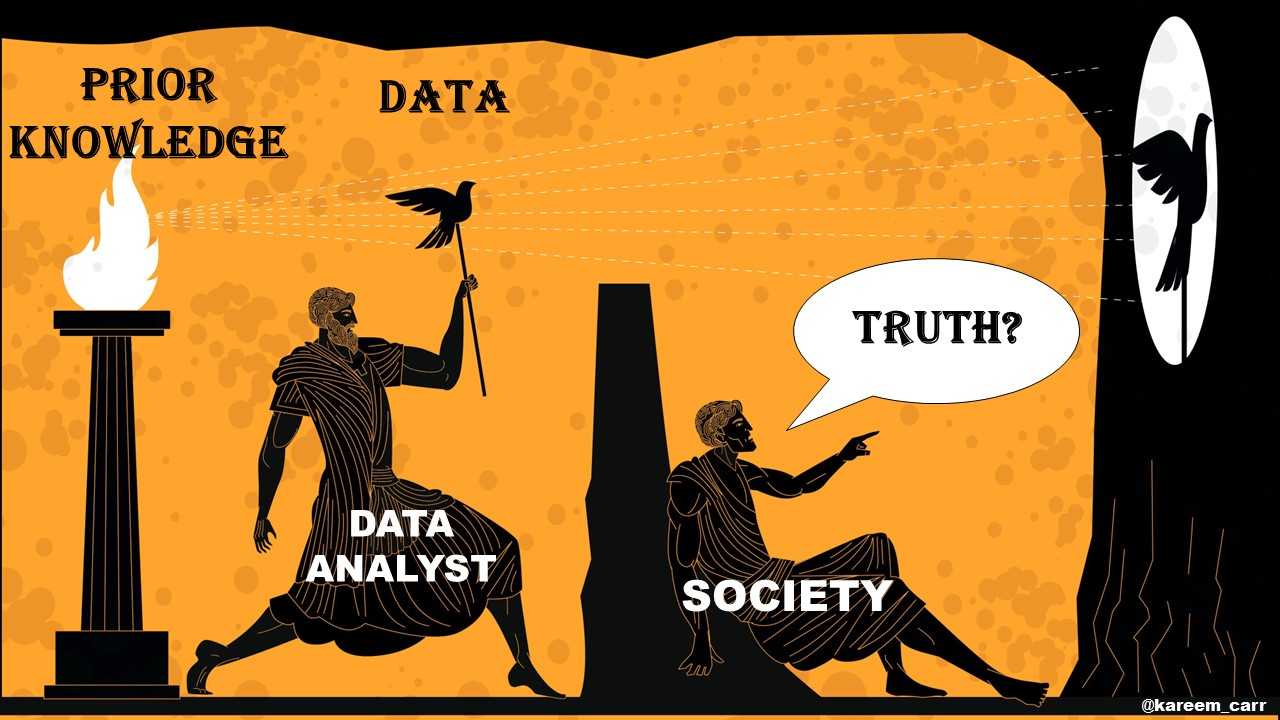
Class goal: translate data into information

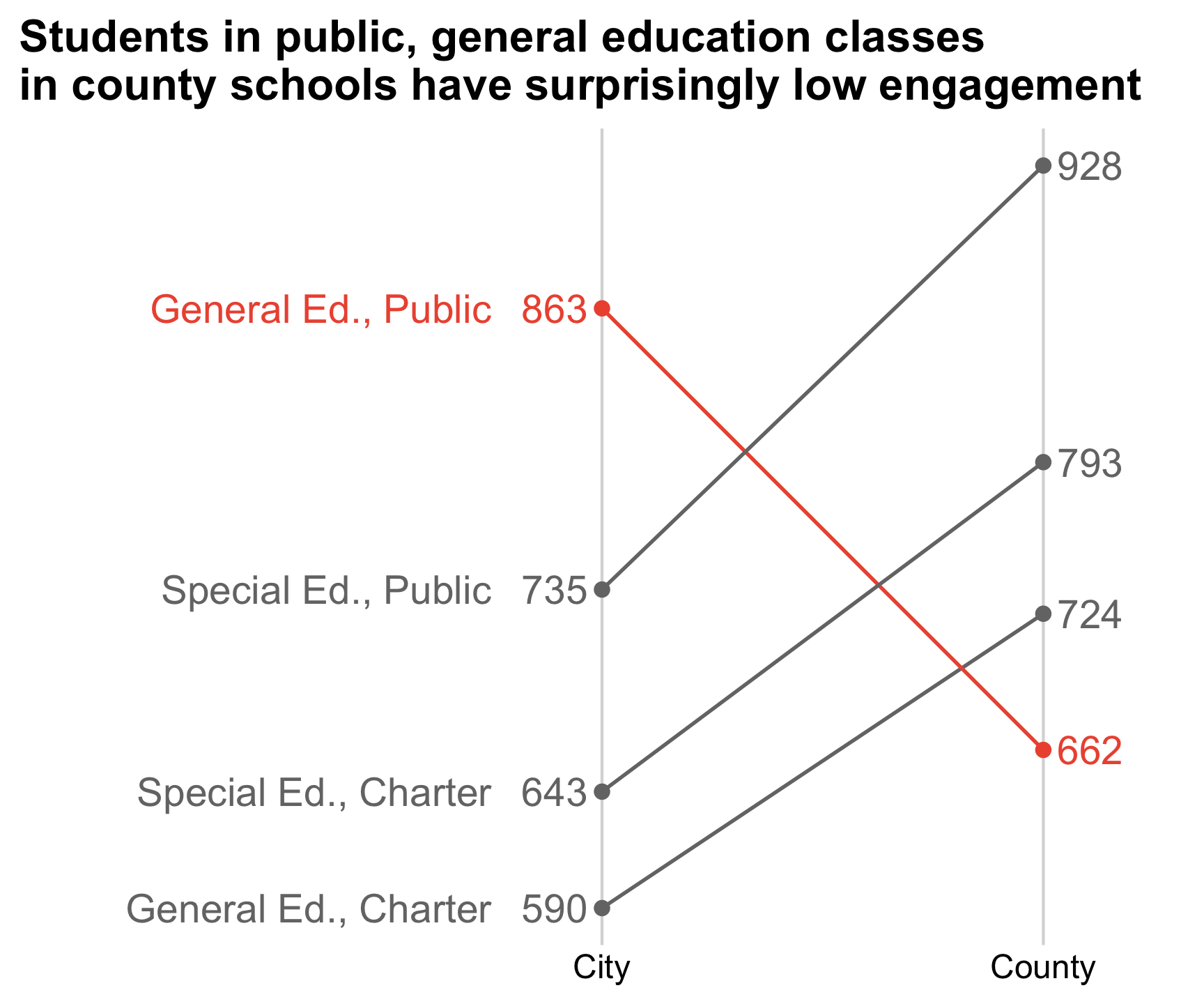
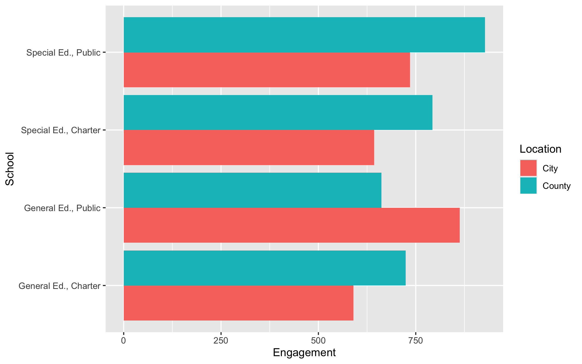
Data

Average student engagement scores

Class	Type	City	County
Special Ed.	Charter	643	793
Special Ed.	Public	735	928
General Ed.	Charter	590	724
General Ed.	Public	863	662

Information

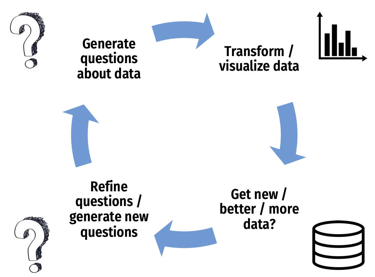
Data exploration: an iterative process

Encode data:

engagement_data <- data.frame(
  City = c(643, 735, 590, 863),
  County = c(793, 928, 724, 662),
  School = c(
    "Special Ed., Charter",
    "Special Ed., Public",
    "General Ed., Charter",
    "General Ed., Public"
  )
)

engagement_data

#>   City County               School
#> 1  643    793 Special Ed., Charter
#> 2  735    928  Special Ed., Public
#> 3  590    724 General Ed., Charter
#> 4  863    662  General Ed., Public

Re-format data for plotting:

engagement_data <- engagement_data %>%
  pivot_longer(
    cols = c(City, County),
    names_to = "Location",
    values_to = "Engagement"
  )

engagement_data

#> # A tibble: 8 × 3
#>   School               Location Engagement
#>   <chr>                <chr>         <dbl>
#> 1 Special Ed., Charter City            643
#> 2 Special Ed., Charter County          793
#> 3 Special Ed., Public  City            735
#> 4 Special Ed., Public  County          928
#> 5 General Ed., Charter City            590
#> 6 General Ed., Charter County          724
#> 7 General Ed., Public  City            863
#> 8 General Ed., Public  County          662

Data exploration: an iterative process

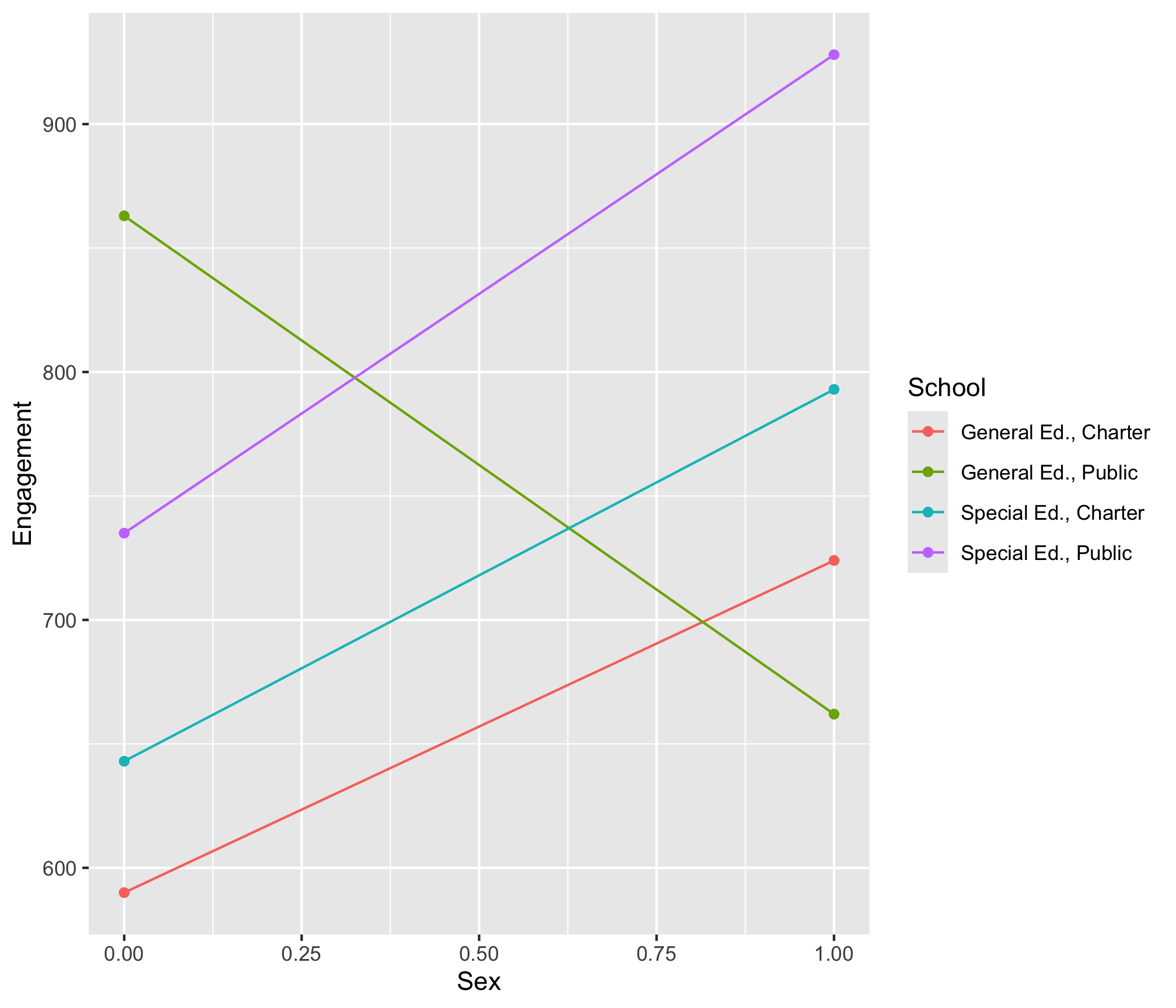
Initial exploratory plotting:

engagement_data %>%
  ggplot() +
  geom_col(
    aes(x = Engagement, y = School, fill = Location),
    position = "dodge"
  )

More exploratory plotting:
highlight difference

Data exploration: an iterative process

Directly label figure:

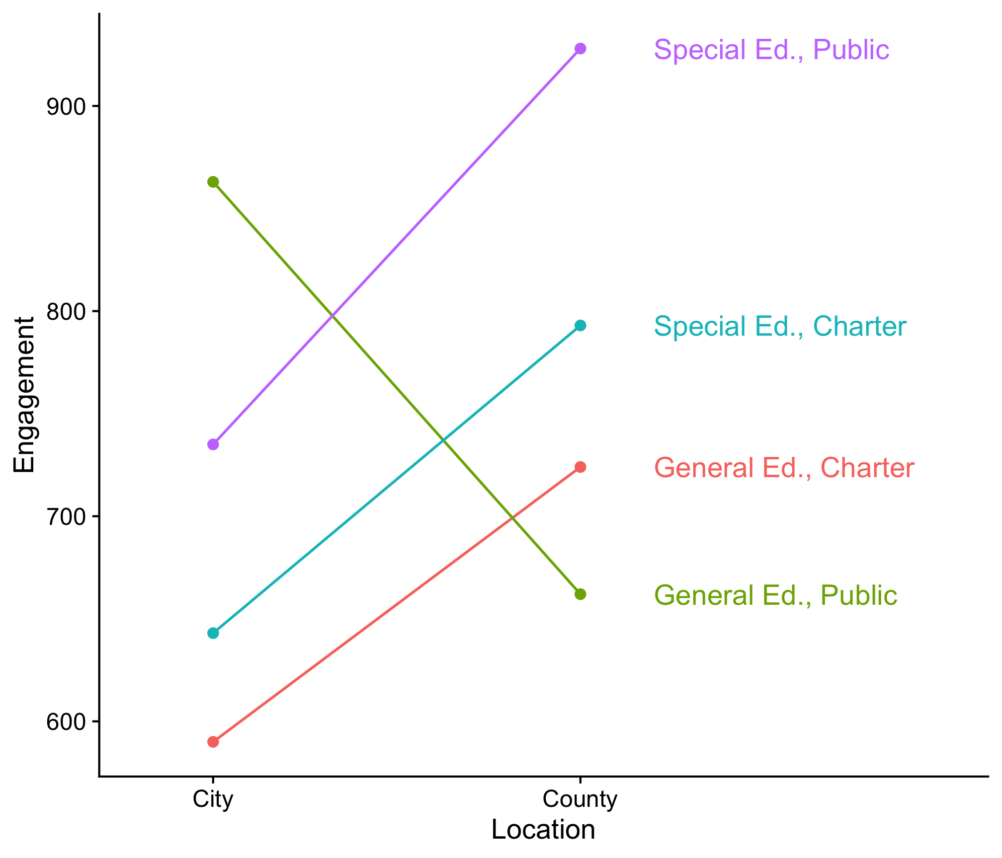
Remove unnecessary axes, change colors, fix labels:

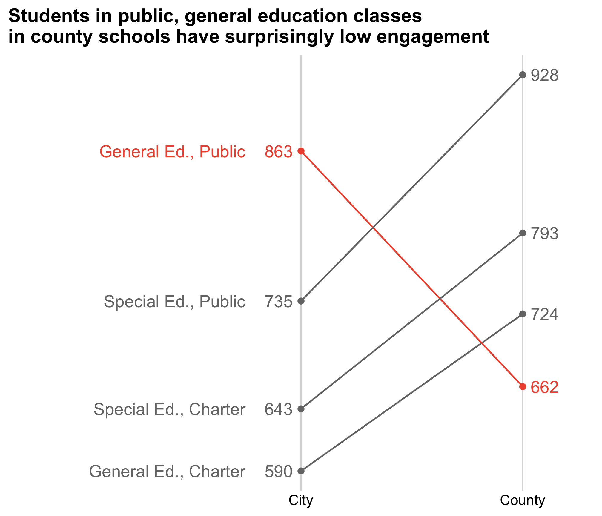
A fully reproducible analysis

Code
Plot

Clean the data

data <- data.frame(
  City = c(643, 735, 590, 863),
  County = c(793, 928, 724, 662),
  School = c(
    "Special Ed., Charter", "Special Ed., Public",
    "General Ed., Charter", "General Ed., Public"
  ),
  Highlight = c(0, 0, 0, 1)
) %>%
  pivot_longer(
    cols = c(City, County), 
    names_to = "Location", 
    values_to = "Engagement"
  ) %>%
  mutate(
    Location = fct_relevel(Location, c("City", "County")),
    Highlight = as.factor(Highlight),
    x = ifelse(Location == "County", 1, 0)
  )

Make the plot

plot <- ggplot(data, aes(
  x = x, y = Engagement, group = School, color = Highlight
)) +
  geom_point() +
  geom_line() +
  scale_color_manual(values = c("#757575", "#ed573e")) +
  labs(
    x = "Sex", y = "Engagement",
    title = "County general-ed classes have low engagement"
  ) +
  scale_x_continuous(
    limits = c(-1.2, 1.2),
    labels = c("City", "County"), breaks = c(0, 1)
  ) +
  geom_text_repel(aes(label = Engagement), size = 5) +
  theme_cowplot() +
  background_grid(major = "x") +
  theme(legend.position = "none")

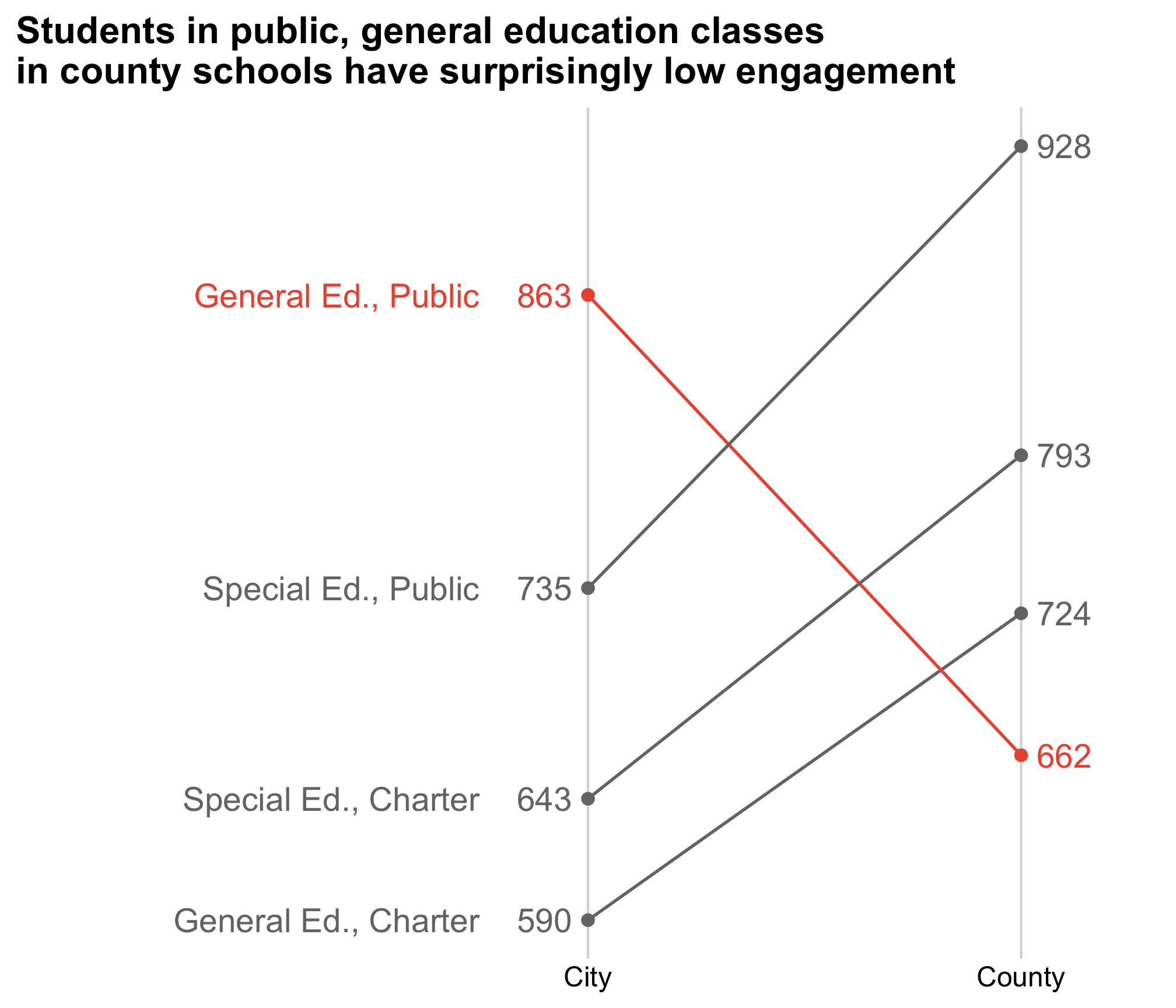
Data exploration: an iterative process

Week 1: Getting Started

1. Course Goal

2. Course Introduction

3. Quarto

4. Workflow & Reading In Data

5. Wrangling Data

6. Visualizing Data

Meet your instructor!

John Helveston, Ph.D.

2025 - Present: Associate Professor, EMSE (w/tenure)
2018 - 2025: Assistant Professor, EMSE
2016-2018: Postdoc at Institute for Sustainable Energy, Boston University
2016: PhD in Engineering & Public Policy at Carnegie Mellon University
2015: MS in Engineering & Public Policy at Carnegie Mellon University
2010: BS in Engineering Science & Mechanics at Virginia Tech
Website: www.jhelvy.com

Meet your tutor!

Lola Nurullaeva

Graduate Teaching Assistant (GTA)
EMSE Ph.D. Student (B.S. SE & M.S. Data Analytics)
Check out her team’s project from 2023

Prerequisites

EMSE 4574 / 6574: Intro to Programming for Analytics

You should be able to:

Use Positron to write basic R commands.
Know the distinctions between different R operators and data types, including numeric, string, and logical data.
Use tidyverse functions to wrangle and manipulate data in R.
Use the ggplot2 library to create plots in R.

Check out R for Analytics Primer

Course website

Everything you need will be on the course website:
https://eda.seas.gwu.edu/2026-Fall/

The schedule is the best starting point

Quizzes (10% of grade)

At the start of class every other week-ish. Make ups only for excused absences (i.e. don’t be late).

5 total, lowest dropped

10 minutes

Why quiz at all? The “retrieval effect” - basically, you have to practice remembering things, otherwise your brain won’t remember them (see the book “Make It Stick: The Science of Successful Learning”)

Assignments

1) Weekly Homework: HW1

2) 3 Mini Projects (due 2 weeks from date assigned)

3) Final Project

Undergrads: Teams of 3 - 4 students

Grads: Teams of 2 students

Item	Due Date
Proposal	Sep 20
Initial Report	Nov 01
Final Report	Dec 06
Presentation	Dec 08

Grades

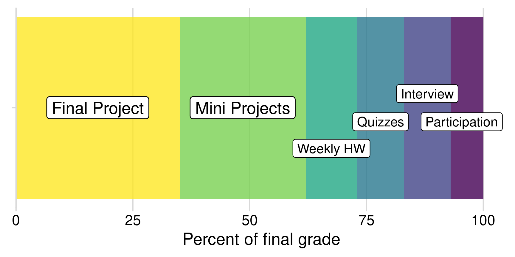
Item	Weight	Notes
Participation / Attendance	7 %	(Yes, I take attendance)
Weekly HW	11 %	Weekly assignment, lowest dropped
Quizzes	10 %	5 quizzes, lowest dropped
Mini Project 1	9 %	Individual assignments
Mini Project 2	9 %
Mini Project 3	9 %
Final Project: Proposal	6 %	Team project
Final Project: Progress Report	6 %
Final Project: Report	17 %
Final Project: Presentation	6 %
Final Interview	10 %	Individual interview

Grades

Course policies

BE NICE

BE HONEST

DON’T CHEAT

Copying is good, stealing is bad

“Plagiarism is trying to pass someone else’s work off as your own. Copying is about reverse-engineering.”

– Austin Kleon, from Steal Like An Artist

Use of AI

We will heavily use AI tools this semester

Large language models (LLMs) are pretty good
Sometimes they suck.
I will grade whatever you submit. It should not suck.

Ways to not have your work suck:

Don’t submit code that doesn’t run (actually run it before submitting it).
Actually read what the AI generates, and don’t submit something you don’t understand. (Ask the LLM to explain why something works or doesn’t work)

Use the approach I teach: agentic workflows (starting next week)

Late submissions

- 3 late days - use them anytime, no questions asked

- No more than 2 late days on any one assignment

- Contact me for special cases

How to succeed in this class

Participate during class!

Start assignments early and read carefully!

Actually read (before class)!

Get sleep and take breaks often!

Ask for help!

Getting Help

Use Slack to ask questions.

Meet with your tutor

Schedule a meeting w/Prof. Helveston (Mon/Tue/Fri)

GW Coders

Course Software

Slack: turn notifications on!

R & Positron (Install both)

Posit Cloud (Register for free!)

Quarto

GitHub Desktop

Break

1. Install everything on the software page

2. Add your GitHub username (NOT GW netID) in
this sheet next to your name

05:00

Week 1: Getting Started

1. Course Goal

2. Course Introduction

3. Quarto

4. Workflow & Reading In Data

5. Wrangling Data

6. Visualizing Data

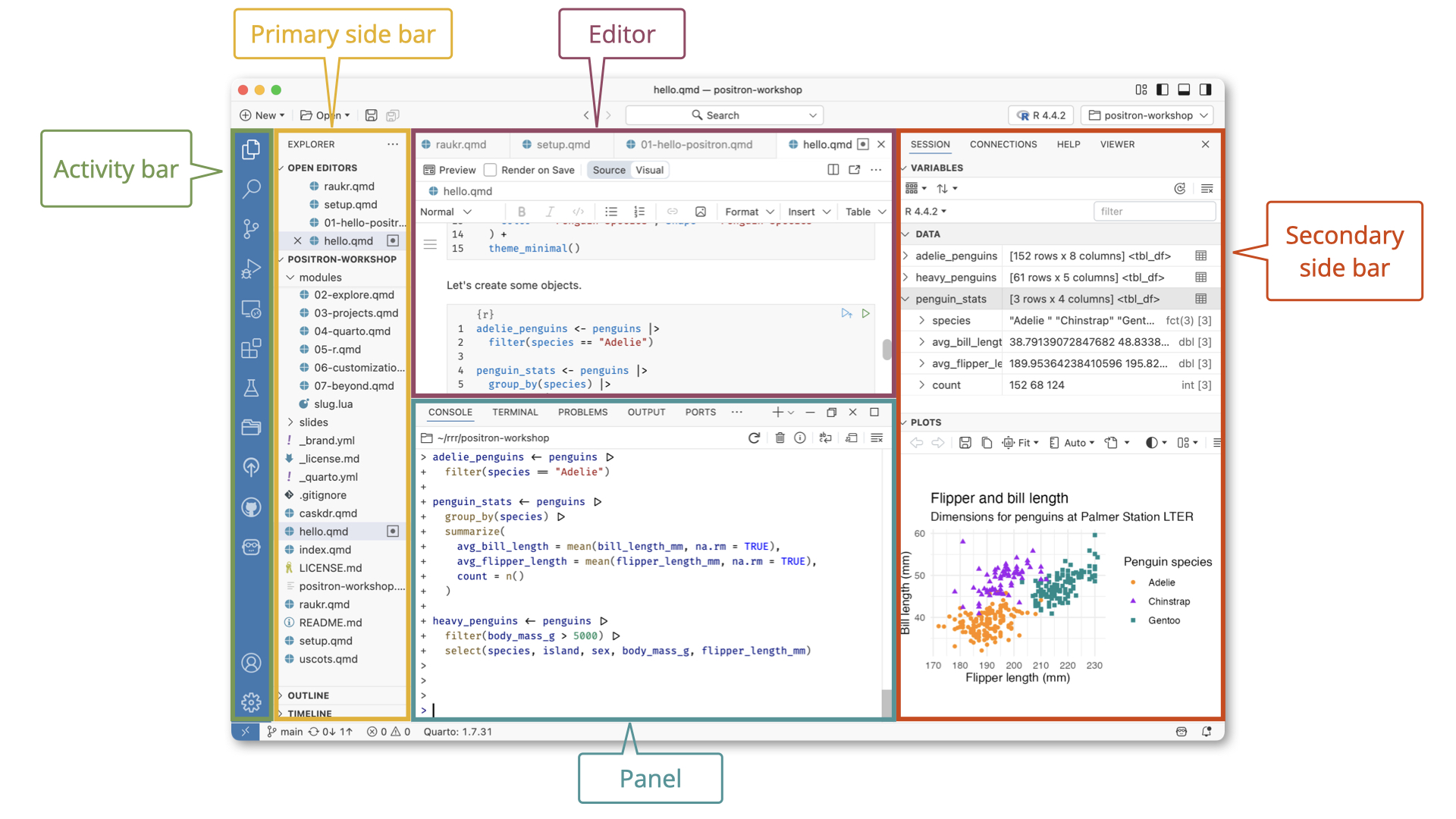
This semester we use Positron

(not RStudio)

Positron Orientation

Quick demo

1. Open `quarto_demo.qmd`

2. Click “Preview”

Anatomy of a .qmd file

Markdown text

R code

Define overall document options in header

Basic html page

---
title: Your title
author: Author name
format: html
---

Add table of contents, change theme

---
title: Your title
author: Author name
toc: true
format:
  html:
    theme: united
---

More on themes at https://quarto.org/docs/output-formats/html-themes.html

Render to multiple outputs

PDF uses LaTeX

---
title: Your title
author: Author name
format: pdf
---

If you don’t have LaTeX on your computer, install tinytex in R:

tinytex::install_tinytex()

Microsoft Word

---
title: Your title
author: Author name
format: docx
---

Anatomy of a .qmd file

Header

Markdown text

R code

Right now, bookmark this! 👇

https://commonmark.org/help/

(When you have 10 minutes, do this! 👇)

https://commonmark.org/help/tutorial/

Headers

# HEADER 1

## HEADER 2

### HEADER 3

#### HEADER 4

##### HEADER 5

###### HEADER 6

HEADER 1

HEADER 2

HEADER 3

HEADER 4

HEADER 5

HEADER 6

Basic Text Formatting

Type this…

normal text
_italic text_
*italic text*
**bold text**
***bold italic text***
~~strikethrough~~
`code text`

..to get this

normal text
italic text
italic text
bold text
bold italic text
~~strikethrough~~
code text

Lists

Bullet list:

- first item
- second item
- third item

first item
second item
third item

Numbered list:

1. first item
2. second item
3. third item

first item
second item
third item

Links

Simple url link to another site:

[Download R](http://www.r-project.org/)

Download R

Anatomy of a .qmd file

Header (think of this as the “settings”)

Markdown text

R code

R Code

Inline code

`r insert code here`

Code chunks

```{r}
insert code here
insert more code here
```

Inline R code

The sum of 3 and 4 is `r 3 + 4`

Produces this:

The sum of 3 and 4 is 7

R Code chunks

This code chunk…

```{r}
library(palmerpenguins)

glimpse(penguins)
```

…will produce this when rendered:

library(palmerpenguins)

glimpse(penguins)

#> Rows: 4
#> Columns: 8
#> $ species           <fct> Adelie, Adelie, Adelie, Adelie
#> $ island            <fct> Torgersen, Torgersen, Torgersen, Torgersen
#> $ bill_length_mm    <dbl> 39.1, 39.5, 40.3, NA
#> $ bill_depth_mm     <dbl> 18.7, 17.4, 18.0, NA
#> $ flipper_length_mm <int> 181, 186, 195, NA
#> $ body_mass_g       <int> 3750, 3800, 3250, NA
#> $ sex               <fct> male, female, female, NA
#> $ year              <int> 2007, 2007, 2007, 2007

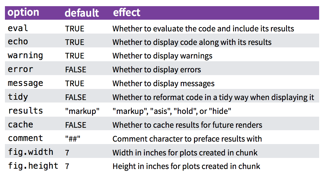
Chunk options

Control what chunks output using options

All options here

Chunk output options

By default, code chunks print code + output

```{r}
#| echo: false

cat('hello world!')
```

Prints only output
(doesn’t show code)

#> hello world!

```{r}
#| eval: false

cat('hello world!')
```

Prints only code
(doesn’t run the code)

cat("hello world!")

```{r}
#| include: false

cat('hello world!')
```

Runs, but doesn’t print anything

A global `setup` chunk 🌍

```{r}
#| label: setup
#| include: false

knitr::opts_chunk$set(
  warning = FALSE,
  message = FALSE,
  fig.width = 7.252,
  fig.height = 4,
  comment = "#>"
)
```

Typically the first chunk
All following chunks will use these options (i.e., sets global chunk options)
You can (and should) use individual chunk options too
Often where I load libraries, etc.

Week 1: Getting Started

1. Course Goal

2. Course Introduction

3. Quarto

4. Workflow & Reading In Data

5. Wrangling Data

6. Visualizing Data

Workflow for reading in data

Open your project folder in Positron - don’t double-click .R files!

Build file paths with file.path() — relative to the folder you opened

path <- file.path("folder", "file.csv")

Import data with these functions:

File type	Function	Library
`.csv`	`read_csv()`	readr
`.txt`	`read.table()`	utils
`.xlsx`	`read_excel()`	readxl

Importing Comma Separated Values (.csv)

Read in .csv files with read_csv():

library(tidyverse)

csvPath <- file.path("data", "milk_production.csv")
milk_production <- read_csv(csvPath)

head(milk_production)

#> # A tibble: 6 × 4
#>   region    state          year milk_produced
#>   <chr>     <chr>         <dbl>         <dbl>
#> 1 Northeast Maine          1970     619000000
#> 2 Northeast New Hampshire  1970     356000000
#> 3 Northeast Vermont        1970    1970000000
#> 4 Northeast Massachusetts  1970     658000000
#> 5 Northeast Rhode Island   1970      75000000
#> 6 Northeast Connecticut    1970     661000000

Importing Text Files (.txt)

Read in .txt files with read.table():

txtPath <- file.path("data", "nasa_global_temps.txt")
global_temps <- read.table(txtPath, skip = 5, header = FALSE)

head(global_temps)

#>     V1    V2    V3
#> 1 1880 -0.15 -0.08
#> 2 1881 -0.07 -0.12
#> 3 1882 -0.10 -0.15
#> 4 1883 -0.16 -0.19
#> 5 1884 -0.27 -0.23
#> 6 1885 -0.32 -0.25

Importing Text Files (.txt)

Read in .txt files with read.table():

txtPath <- file.path("data", "nasa_global_temps.txt")
global_temps <- read.table(txtPath, skip = 5, header = FALSE)
names(global_temps) <- c("year", "no_smoothing", "loess") # Add header

head(global_temps)

#>   year no_smoothing loess
#> 1 1880        -0.15 -0.08
#> 2 1881        -0.07 -0.12
#> 3 1882        -0.10 -0.15
#> 4 1883        -0.16 -0.19
#> 5 1884        -0.27 -0.23
#> 6 1885        -0.32 -0.25

Importing Excel Files (.xlsx)

Read in .xlsx files with read_excel():

library(readxl)

xlsxPath <- file.path("data", "pv_cell_production.xlsx")
pv_cells <- read_excel(xlsxPath, sheet = "Cell Prod by Country", skip = 2)

glimpse(pv_cells)

#> Rows: 6
#> Columns: 10
#> $ Year            <chr> NA, NA, "1995", "1996", "1997", "1998"
#> $ China           <chr> "Megawatts", NA, "NA", "NA", "NA", "NA"
#> $ Taiwan          <chr> NA, NA, "NA", "NA", "NA", "NA"
#> $ Japan           <dbl> NA, NA, 16.4, 21.2, 35.0, 49.0
#> $ Malaysia        <chr> NA, NA, "NA", "NA", "NA", "NA"
#> $ Germany         <chr> NA, NA, "NA", "NA", "NA", "NA"
#> $ `South Korea`   <chr> NA, NA, "NA", "NA", "NA", "NA"
#> $ `United States` <dbl> NA, NA, 34.75, 38.85, 51.00, 53.70
#> $ Others          <chr> NA, NA, "NA", "NA", "NA", "NA"
#> $ World           <dbl> NA, NA, 77.6, 88.6, 125.8, 154.9

Importing Excel Files (.xlsx)

Read in .xlsx files with read_excel():

library(readxl)

xlsxPath <- file.path("data", "pv_cell_production.xlsx")
pv_cells <- read_excel(xlsxPath, sheet = "Cell Prod by Country", skip = 2) %>%
  mutate(Year = as.numeric(Year)) %>% # Convert "non-years" to NA
  filter(!is.na(Year)) # Drop NA rows in Year

glimpse(pv_cells)

#> Rows: 6
#> Columns: 10
#> $ Year            <dbl> 1995, 1996, 1997, 1998, 1999, 2000
#> $ China           <chr> "NA", "NA", "NA", "NA", "NA", "2.5"
#> $ Taiwan          <chr> "NA", "NA", "NA", "NA", "NA", "NA"
#> $ Japan           <dbl> 16.4, 21.2, 35.0, 49.0, 80.0, 128.6
#> $ Malaysia        <chr> "NA", "NA", "NA", "NA", "NA", "NA"
#> $ Germany         <chr> "NA", "NA", "NA", "NA", "NA", "22.5"
#> $ `South Korea`   <chr> "NA", "NA", "NA", "NA", "NA", "NA"
#> $ `United States` <dbl> 34.75, 38.85, 51.00, 53.70, 60.80, 75.00
#> $ Others          <chr> "NA", "NA", "NA", "NA", "NA", "48.200000000000017"
#> $ World           <dbl> 77.6, 88.6, 125.8, 154.9, 201.3, 276.8

Your turn

Open the practice.qmd file.

Write code to import the following data files from the “data” folder:

For lotr_words.csv, call the data frame lotr
For north_america_bear_killings.txt, call the data frame bears
For uspto_clean_energy_patents.xlsx, call the data frame patents

10:00

Week 1: Getting Started

1. Course Goal

2. Course Introduction

3. Quarto

4. Workflow & Reading In Data

5. Wrangling Data

6. Visualizing Data

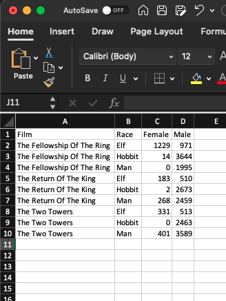
The data frame…
in Excel

The data frame…
in

lotr

#> # A tibble: 18 × 4
#>    film                       race   gender word_count
#>    <chr>                      <chr>  <chr>       <dbl>
#>  1 The Fellowship Of The Ring Elf    Female       1229
#>  2 The Fellowship Of The Ring Elf    Male          971
#>  3 The Fellowship Of The Ring Hobbit Female         14
#>  4 The Fellowship Of The Ring Hobbit Male         3644
#>  5 The Fellowship Of The Ring Man    Female          0
#>  6 The Fellowship Of The Ring Man    Male         1995
#>  7 The Return Of The King     Elf    Female        183
#>  8 The Return Of The King     Elf    Male          510
#>  9 The Return Of The King     Hobbit Female          2
#> 10 The Return Of The King     Hobbit Male         2673
#> 11 The Return Of The King     Man    Female        268
#> 12 The Return Of The King     Man    Male         2459
#> 13 The Two Towers             Elf    Female        331
#> 14 The Two Towers             Elf    Male          513
#> 15 The Two Towers             Hobbit Female          0
#> 16 The Two Towers             Hobbit Male         2463
#> 17 The Two Towers             Man    Female        401
#> 18 The Two Towers             Man    Male         3589

Columns: Vectors of values (must be same data type)

Extract a column using $

lotr$race

#>  [1] "Elf"    "Elf"    "Hobbit" "Hobbit" "Man"    "Man"    "Elf"    "Elf"    "Hobbit" "Hobbit" "Man"    "Man"    "Elf"    "Elf"    "Hobbit" "Hobbit" "Man"    "Man"

Columns: Vectors of values (must be same data type)

Can also use brackets:

lotr$race

#>  [1] "Elf"    "Elf"    "Hobbit" "Hobbit" "Man"    "Man"    "Elf"    "Elf"    "Hobbit" "Hobbit" "Man"    "Man"    "Elf"    "Elf"    "Hobbit" "Hobbit" "Man"    "Man"

lotr[, 2]

#> # A tibble: 18 × 1
#>    race  
#>    <chr> 
#>  1 Elf   
#>  2 Elf   
#>  3 Hobbit
#>  4 Hobbit
#>  5 Man   
#>  6 Man   
#>  7 Elf   
#>  8 Elf   
#>  9 Hobbit
#> 10 Hobbit
#> 11 Man   
#> 12 Man   
#> 13 Elf   
#> 14 Elf   
#> 15 Hobbit
#> 16 Hobbit
#> 17 Man   
#> 18 Man

Rows: Information about individual observations

Information about the first row:

lotr[1, ]

#> # A tibble: 1 × 4
#>   film                       race  gender word_count
#>   <chr>                      <chr> <chr>       <dbl>
#> 1 The Fellowship Of The Ring Elf   Female       1229

Information about rows 1 & 2:

lotr[1:2, ]

#> # A tibble: 2 × 4
#>   film                       race  gender word_count
#>   <chr>                      <chr> <chr>       <dbl>
#> 1 The Fellowship Of The Ring Elf   Female       1229
#> 2 The Fellowship Of The Ring Elf   Male          971

Quick Practice

Read in the data.csv file in the “data” folder:

data <- read_csv(file.path("data", "data.csv"))

Now answer these questions:

How many rows and columns are in the data frame?
What type of data is each column?
Preview the different columns - what do you think this data is about? What might one row represent?
How many unique airlines are in the data frame?
What is the shortest and longest air time for any one flight in the data frame?

The tidyverse: `stringr` + `dplyr` + `readr` + `ggplot2` + …

Art by Allison Horst

The main `dplyr` “verbs”

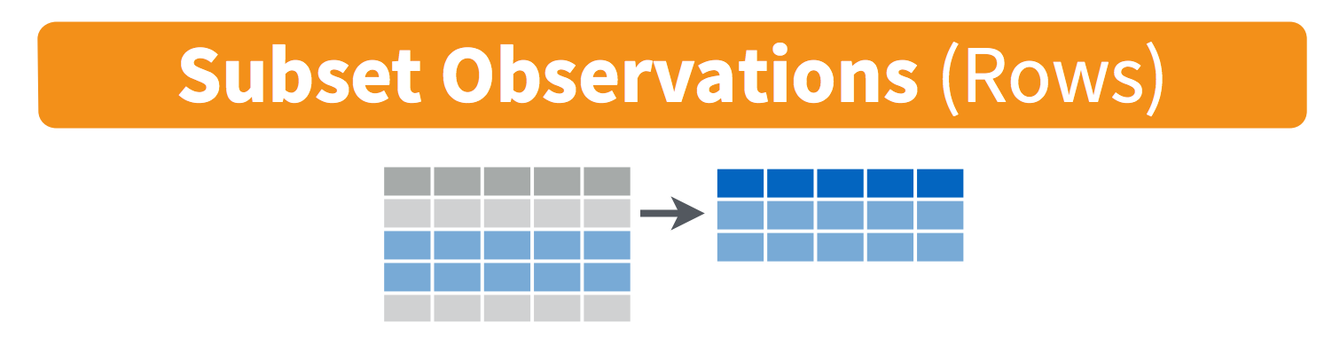
“Verb”	What it does
`select()`	Select columns by name
`filter()`	Keep rows that match criteria
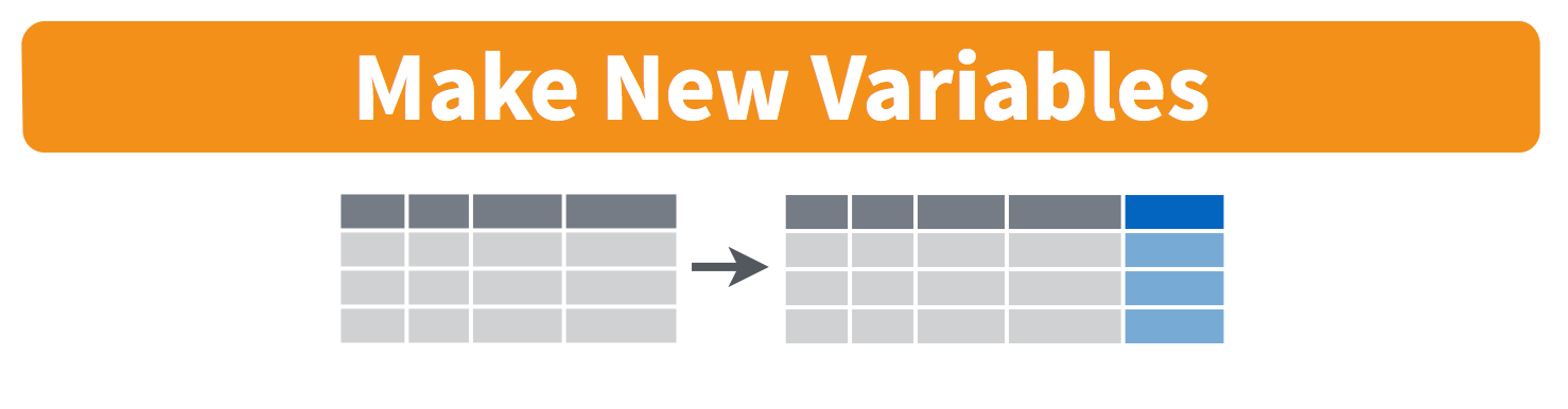
`arrange()`	Sort rows based on column(s)
`mutate()`	Create new columns
`summarize()`	Create summary values

Core `tidyverse` concept:
Chain functions together with “pipes”

`%>%`

Think of the words “…and then…”

data %>%
  do_something() %>%
  do_something_else()

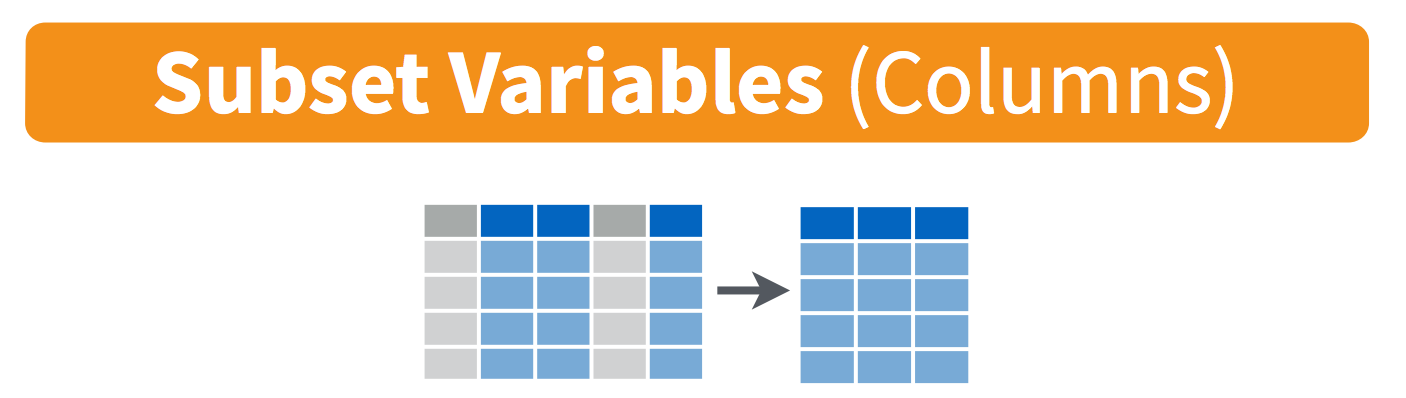
Select columns with `select()`

Select the columns film & race

lotr %>%
  select(film, race)

#> # A tibble: 18 × 2
#>    film                       race  
#>    <chr>                      <chr> 
#>  1 The Fellowship Of The Ring Elf   
#>  2 The Fellowship Of The Ring Elf   
#>  3 The Fellowship Of The Ring Hobbit
#>  4 The Fellowship Of The Ring Hobbit
#>  5 The Fellowship Of The Ring Man   
#>  6 The Fellowship Of The Ring Man   
#>  7 The Return Of The King     Elf   
#>  8 The Return Of The King     Elf   
#>  9 The Return Of The King     Hobbit
#> 10 The Return Of The King     Hobbit
#> 11 The Return Of The King     Man   
#> 12 The Return Of The King     Man   
#> 13 The Two Towers             Elf   
#> 14 The Two Towers             Elf   
#> 15 The Two Towers             Hobbit
#> 16 The Two Towers             Hobbit
#> 17 The Two Towers             Man   
#> 18 The Two Towers             Man

Select columns with `select()`

Use the - sign to drop columns

lotr %>%
  select(-film)

#> # A tibble: 18 × 3
#>    race   gender word_count
#>    <chr>  <chr>       <dbl>
#>  1 Elf    Female       1229
#>  2 Elf    Male          971
#>  3 Hobbit Female         14
#>  4 Hobbit Male         3644
#>  5 Man    Female          0
#>  6 Man    Male         1995
#>  7 Elf    Female        183
#>  8 Elf    Male          510
#>  9 Hobbit Female          2
#> 10 Hobbit Male         2673
#> 11 Man    Female        268
#> 12 Man    Male         2459
#> 13 Elf    Female        331
#> 14 Elf    Male          513
#> 15 Hobbit Female          0
#> 16 Hobbit Male         2463
#> 17 Man    Female        401
#> 18 Man    Male         3589

Filter for rows with `filter()`

Keep only the rows with Elf characters

lotr %>%
  filter(race == "Elf")

#> # A tibble: 6 × 4
#>   film                       race  gender word_count
#>   <chr>                      <chr> <chr>       <dbl>
#> 1 The Fellowship Of The Ring Elf   Female       1229
#> 2 The Fellowship Of The Ring Elf   Male          971
#> 3 The Return Of The King     Elf   Female        183
#> 4 The Return Of The King     Elf   Male          510
#> 5 The Two Towers             Elf   Female        331
#> 6 The Two Towers             Elf   Male          513

Filter for rows with `filter()`

Keep only the rows with Elf or Hobbit characters

lotr %>%
  filter((race == "Elf") | (race == "Hobbit"))

#> # A tibble: 12 × 4
#>    film                       race   gender word_count
#>    <chr>                      <chr>  <chr>       <dbl>
#>  1 The Fellowship Of The Ring Elf    Female       1229
#>  2 The Fellowship Of The Ring Elf    Male          971
#>  3 The Fellowship Of The Ring Hobbit Female         14
#>  4 The Fellowship Of The Ring Hobbit Male         3644
#>  5 The Return Of The King     Elf    Female        183
#>  6 The Return Of The King     Elf    Male          510
#>  7 The Return Of The King     Hobbit Female          2
#>  8 The Return Of The King     Hobbit Male         2673
#>  9 The Two Towers             Elf    Female        331
#> 10 The Two Towers             Elf    Male          513
#> 11 The Two Towers             Hobbit Female          0
#> 12 The Two Towers             Hobbit Male         2463

Filter for rows with `filter()`

Keep only the rows with Elf or Hobbit characters

lotr %>%
  filter(race %in% c("Elf", "Hobbit"))

#> # A tibble: 12 × 4
#>    film                       race   gender word_count
#>    <chr>                      <chr>  <chr>       <dbl>
#>  1 The Fellowship Of The Ring Elf    Female       1229
#>  2 The Fellowship Of The Ring Elf    Male          971
#>  3 The Fellowship Of The Ring Hobbit Female         14
#>  4 The Fellowship Of The Ring Hobbit Male         3644
#>  5 The Return Of The King     Elf    Female        183
#>  6 The Return Of The King     Elf    Male          510
#>  7 The Return Of The King     Hobbit Female          2
#>  8 The Return Of The King     Hobbit Male         2673
#>  9 The Two Towers             Elf    Female        331
#> 10 The Two Towers             Elf    Male          513
#> 11 The Two Towers             Hobbit Female          0
#> 12 The Two Towers             Hobbit Male         2463

Logic operators for `filter()`

Description	Example
Values greater than 1	`value > 1`
Values greater than or equal to 1	`value >= 1`
Values less than 1	`value < 1`
Values less than or equal to 1	`value <= 1`
Values equal to 1	`value == 1`
Values not equal to 1	`value != 1`
Values in the set c(1, 4)	`value %in% c(1, 4)`

Combine `filter()` and `select()`

Keep only the rows with Elf characters that spoke more than 1000 words, then select everything but the race column

lotr %>%
  filter((race == "Elf") & (word_count > 1000)) %>%
  select(-race)

#> # A tibble: 1 × 3
#>   film                       gender word_count
#>   <chr>                      <chr>       <dbl>
#> 1 The Fellowship Of The Ring Female       1229

Create new variables with `mutate()`

Create a new variable, word1000 which is TRUE if the character spoke 1,000 or more words

lotr %>%
  mutate(word1000 = word_count >= 1000)

#> # A tibble: 18 × 5
#>    film                       race   gender word_count word1000
#>    <chr>                      <chr>  <chr>       <dbl> <lgl>   
#>  1 The Fellowship Of The Ring Elf    Female       1229 TRUE    
#>  2 The Fellowship Of The Ring Elf    Male          971 FALSE   
#>  3 The Fellowship Of The Ring Hobbit Female         14 FALSE   
#>  4 The Fellowship Of The Ring Hobbit Male         3644 TRUE    
#>  5 The Fellowship Of The Ring Man    Female          0 FALSE   
#>  6 The Fellowship Of The Ring Man    Male         1995 TRUE    
#>  7 The Return Of The King     Elf    Female        183 FALSE   
#>  8 The Return Of The King     Elf    Male          510 FALSE   
#>  9 The Return Of The King     Hobbit Female          2 FALSE   
#> 10 The Return Of The King     Hobbit Male         2673 TRUE    
#> 11 The Return Of The King     Man    Female        268 FALSE   
#> 12 The Return Of The King     Man    Male         2459 TRUE    
#> 13 The Two Towers             Elf    Female        331 FALSE   
#> 14 The Two Towers             Elf    Male          513 FALSE   
#> 15 The Two Towers             Hobbit Female          0 FALSE   
#> 16 The Two Towers             Hobbit Male         2463 TRUE    
#> 17 The Two Towers             Man    Female        401 FALSE   
#> 18 The Two Towers             Man    Male         3589 TRUE

Handling if/else conditions

`ifelse(<condition>, <if TRUE>, <else>)`

lotr %>%
  mutate(word1000 = ifelse(word_count >= 1000, TRUE, FALSE))

#> # A tibble: 18 × 5
#>    film                       race   gender word_count word1000
#>    <chr>                      <chr>  <chr>       <dbl> <lgl>   
#>  1 The Fellowship Of The Ring Elf    Female       1229 TRUE    
#>  2 The Fellowship Of The Ring Elf    Male          971 FALSE   
#>  3 The Fellowship Of The Ring Hobbit Female         14 FALSE   
#>  4 The Fellowship Of The Ring Hobbit Male         3644 TRUE    
#>  5 The Fellowship Of The Ring Man    Female          0 FALSE   
#>  6 The Fellowship Of The Ring Man    Male         1995 TRUE    
#>  7 The Return Of The King     Elf    Female        183 FALSE   
#>  8 The Return Of The King     Elf    Male          510 FALSE   
#>  9 The Return Of The King     Hobbit Female          2 FALSE   
#> 10 The Return Of The King     Hobbit Male         2673 TRUE    
#> 11 The Return Of The King     Man    Female        268 FALSE   
#> 12 The Return Of The King     Man    Male         2459 TRUE    
#> 13 The Two Towers             Elf    Female        331 FALSE   
#> 14 The Two Towers             Elf    Male          513 FALSE   
#> 15 The Two Towers             Hobbit Female          0 FALSE   
#> 16 The Two Towers             Hobbit Male         2463 TRUE    
#> 17 The Two Towers             Man    Female        401 FALSE   
#> 18 The Two Towers             Man    Male         3589 TRUE

Sort data frame with `arrange()`

Sort the lotr data frame by word_count

lotr %>%
  arrange(word_count)

#> # A tibble: 18 × 4
#>    film                       race   gender word_count
#>    <chr>                      <chr>  <chr>       <dbl>
#>  1 The Fellowship Of The Ring Man    Female          0
#>  2 The Two Towers             Hobbit Female          0
#>  3 The Return Of The King     Hobbit Female          2
#>  4 The Fellowship Of The Ring Hobbit Female         14
#>  5 The Return Of The King     Elf    Female        183
#>  6 The Return Of The King     Man    Female        268
#>  7 The Two Towers             Elf    Female        331
#>  8 The Two Towers             Man    Female        401
#>  9 The Return Of The King     Elf    Male          510
#> 10 The Two Towers             Elf    Male          513
#> 11 The Fellowship Of The Ring Elf    Male          971
#> 12 The Fellowship Of The Ring Elf    Female       1229
#> 13 The Fellowship Of The Ring Man    Male         1995
#> 14 The Return Of The King     Man    Male         2459
#> 15 The Two Towers             Hobbit Male         2463
#> 16 The Return Of The King     Hobbit Male         2673
#> 17 The Two Towers             Man    Male         3589
#> 18 The Fellowship Of The Ring Hobbit Male         3644

Sort data frame with `arrange()`

Use the desc() function to sort in descending order

lotr %>%
  arrange(desc(word_count))

#> # A tibble: 18 × 4
#>    film                       race   gender word_count
#>    <chr>                      <chr>  <chr>       <dbl>
#>  1 The Fellowship Of The Ring Hobbit Male         3644
#>  2 The Two Towers             Man    Male         3589
#>  3 The Return Of The King     Hobbit Male         2673
#>  4 The Two Towers             Hobbit Male         2463
#>  5 The Return Of The King     Man    Male         2459
#>  6 The Fellowship Of The Ring Man    Male         1995
#>  7 The Fellowship Of The Ring Elf    Female       1229
#>  8 The Fellowship Of The Ring Elf    Male          971
#>  9 The Two Towers             Elf    Male          513
#> 10 The Return Of The King     Elf    Male          510
#> 11 The Two Towers             Man    Female        401
#> 12 The Two Towers             Elf    Female        331
#> 13 The Return Of The King     Man    Female        268
#> 14 The Return Of The King     Elf    Female        183
#> 15 The Fellowship Of The Ring Hobbit Female         14
#> 16 The Return Of The King     Hobbit Female          2
#> 17 The Fellowship Of The Ring Man    Female          0
#> 18 The Two Towers             Hobbit Female          0

10:00

Your turn

Read in the data.csv file in the “data” folder:

data <- read_csv(file.path("data", "data.csv"))

Create a new data frame, flights_fall, that contains only flights that departed in the fall semester.
Create a new data frame, flights_dc, that contains only flights that flew to DC airports (Reagan or Dulles).
Create a new data frame, flights_dc_carrier, that contains only flights that flew to DC airports (Reagan or Dulles) and only the columns about the month and airline.
How many unique airlines were flying to DC airports in July?
Create a new variable, speed, in miles per hour using the time (minutes) and distance (miles) variables.
Which flight flew the fastest?
Remove rows that have NA for air_time and re-arrange the resulting data frame based on the longest air time and longest flight distance.

Week 1: Getting Started

1. Course Goal

2. Course Introduction

3. Quarto

4. Workflow & Reading In Data

5. Wrangling Data

6. Visualizing Data

“Grammar of Graphics”

Concept developed by Leland Wilkinson (1999)

ggplot2 package developed by Hadley Wickham (2005)

Making plot layers with ggplot2

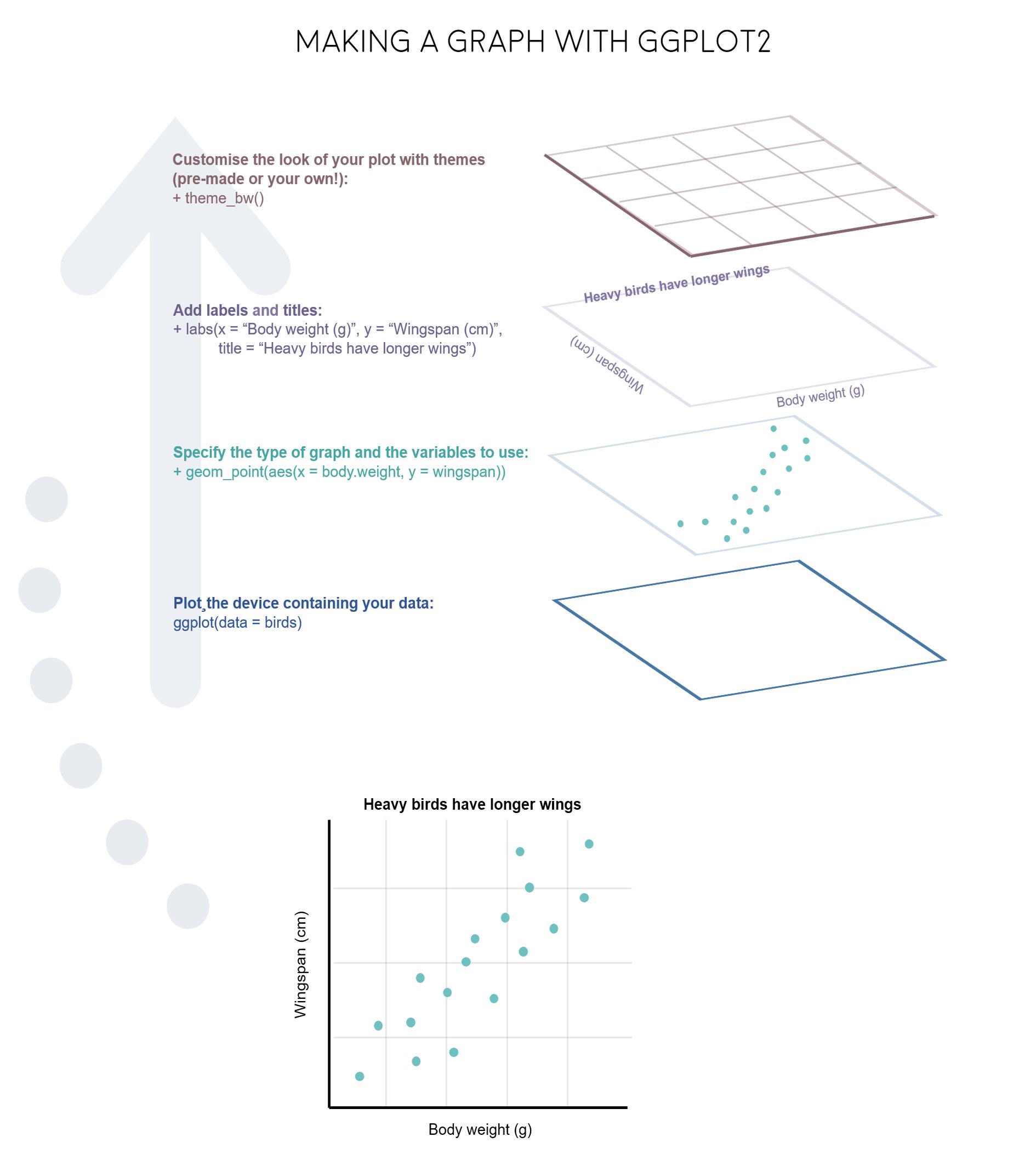
1. The data

2. The aesthetic mapping (what goes on the axes?)

3. The geometries (points? bars? etc.)

4. The annotations / labels

5. The theme

Layer 1: The data

head(mpg)

#> # A tibble: 6 × 11
#>   manufacturer model displ  year   cyl trans      drv     cty   hwy fl    class  
#>   <chr>        <chr> <dbl> <int> <int> <chr>      <chr> <int> <int> <chr> <chr>  
#> 1 audi         a4      1.8  1999     4 auto(l5)   f        18    29 p     compact
#> 2 audi         a4      1.8  1999     4 manual(m5) f        21    29 p     compact
#> 3 audi         a4      2    2008     4 manual(m6) f        20    31 p     compact
#> 4 audi         a4      2    2008     4 auto(av)   f        21    30 p     compact
#> 5 audi         a4      2.8  1999     6 auto(l5)   f        16    26 p     compact
#> 6 audi         a4      2.8  1999     6 manual(m5) f        18    26 p     compact

Layer 1: The data

The ggplot() function initializes the plot with whatever data you’re using

mpg %>%
  ggplot()

Layer 2: The aesthetic mapping

The aes() function determines which variables will be mapped to the geometries
(e.g. the axes)

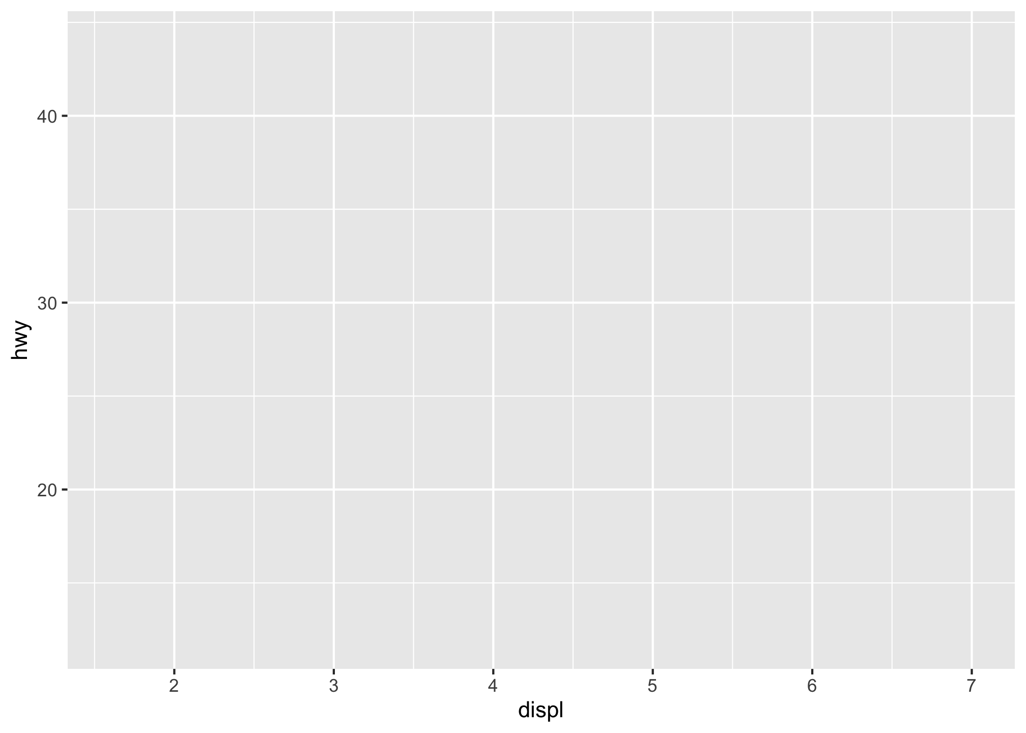
mpg %>%
  ggplot(aes(x = displ, y = hwy))

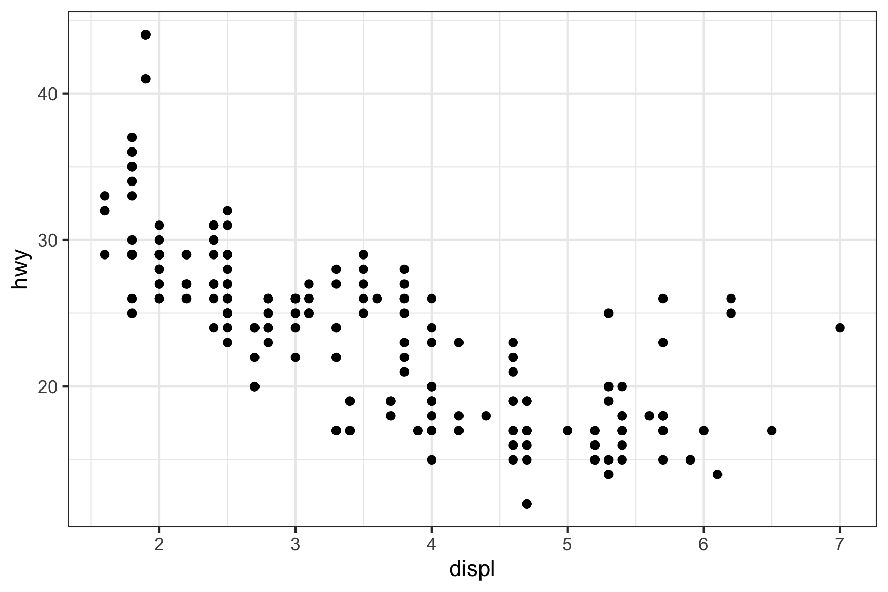
Layer 3: The geometries

Use + to add geometries, e.g. geom_point() for points

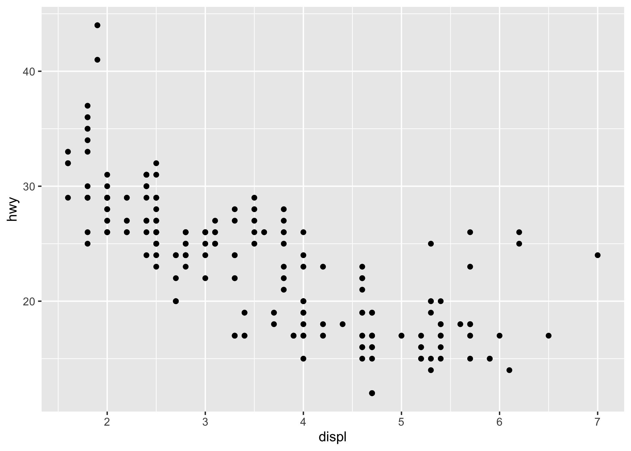
mpg %>%
  ggplot(aes(x = displ, y = hwy)) +
  geom_point()

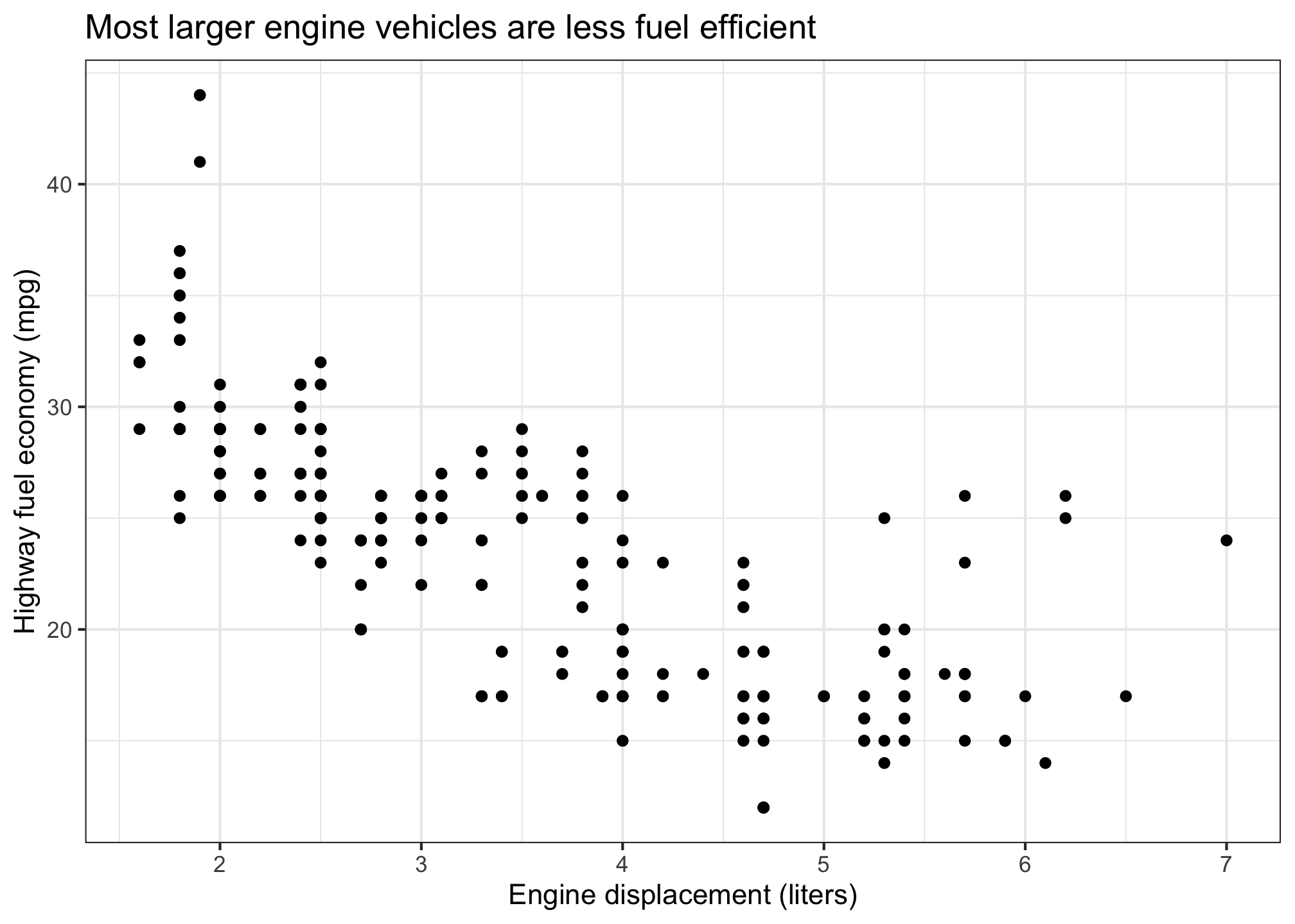
Layer 4: The annotations / labels

Use labs() to modify most labels

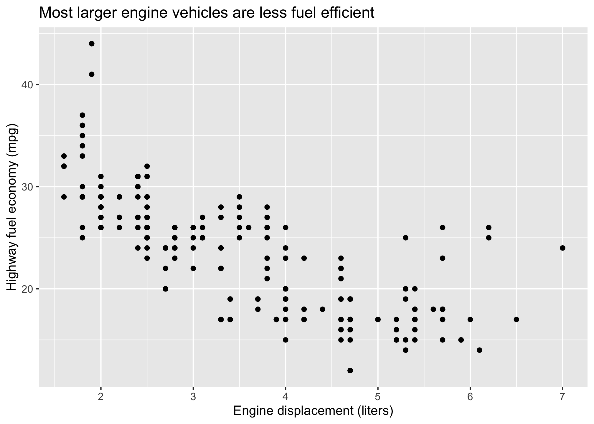
mpg %>%
  ggplot(aes(x = displ, y = hwy)) +
  geom_point() +
  labs(
    x = "Engine displacement (liters)",
    y = "Highway fuel economy (mpg)",
    title = "Most larger engine vehicles are less fuel efficient"
  )

Layer 5: The theme

mpg %>%
  ggplot(aes(x = displ, y = hwy)) +
  geom_point() +
  labs(
    x = "Engine displacement (liters)",
    y = "Highway fuel economy (mpg)",
    title = "Most larger engine vehicles are less fuel efficient"
  ) +
  theme_bw()

Common themes

theme_bw()

mpg %>%
  ggplot(aes(x = displ, y = hwy)) +
  geom_point() +
  theme_bw()

theme_minimal()

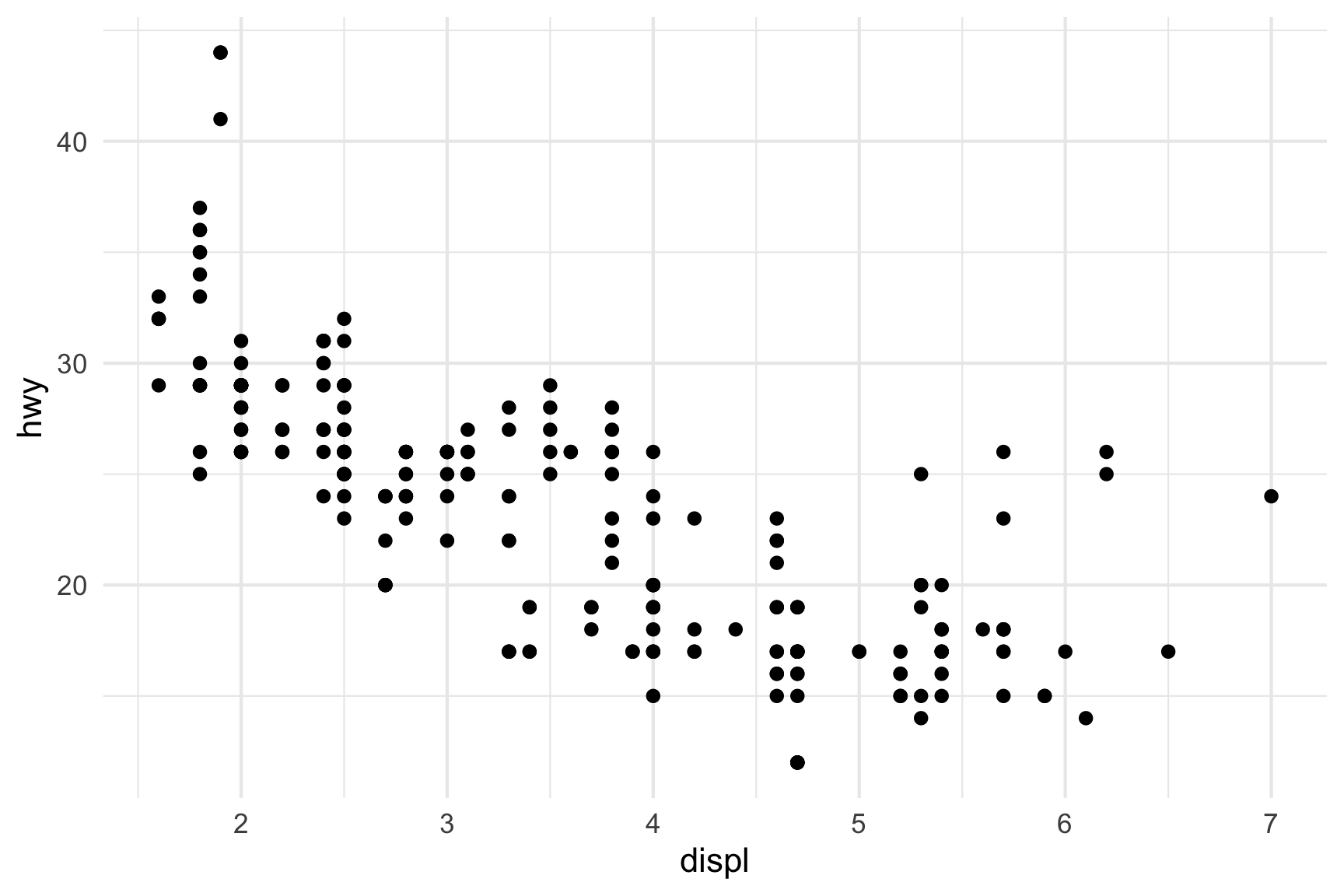
mpg %>%
  ggplot(aes(x = displ, y = hwy)) +
  geom_point() +
  theme_minimal()

Common themes

theme_classic()

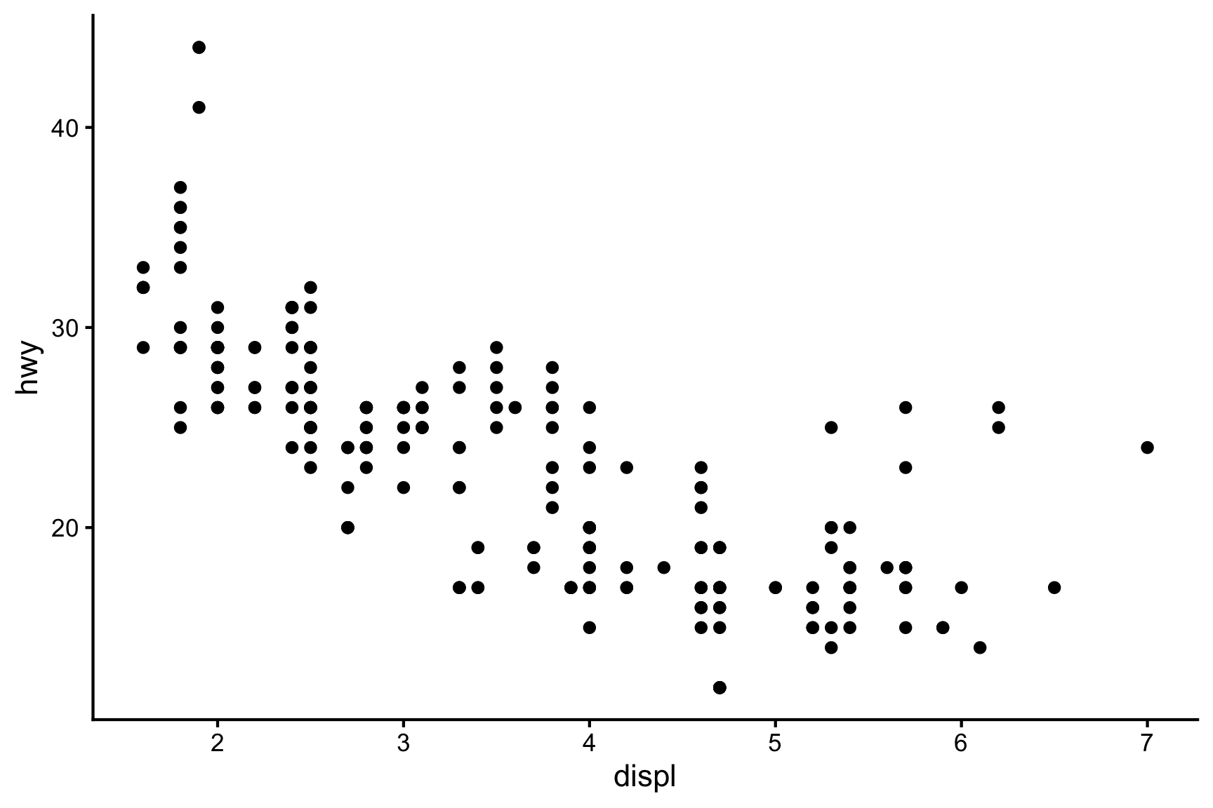
mpg %>%
  ggplot(aes(x = displ, y = hwy)) +
  geom_point() +
  theme_classic()

theme_void()

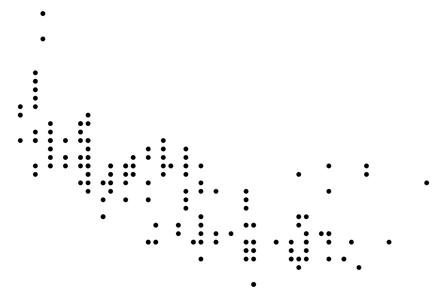
mpg %>%
  ggplot(aes(x = displ, y = hwy)) +
  geom_point() +
  theme_void()

15:00

Your turn

Open practice.qmd

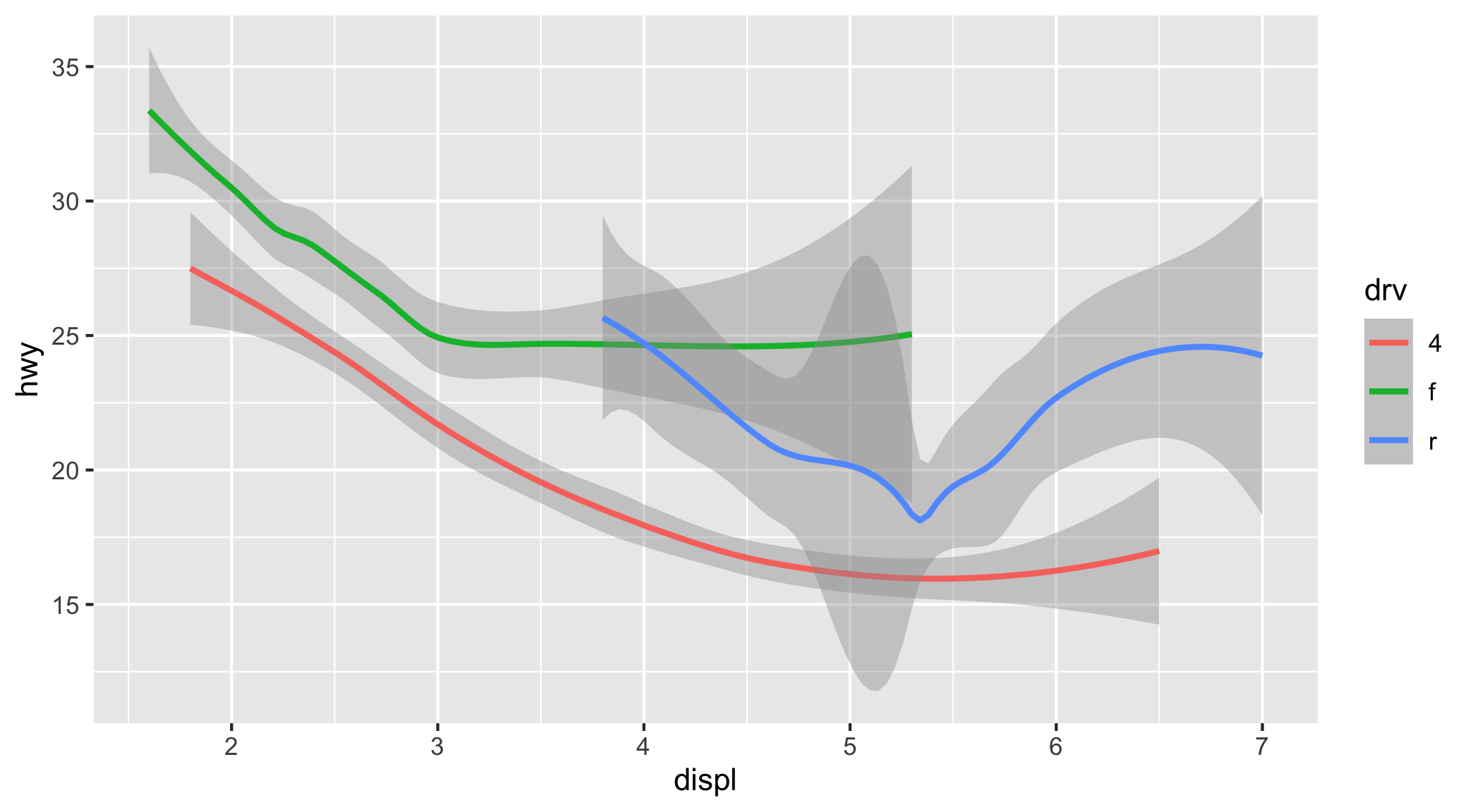
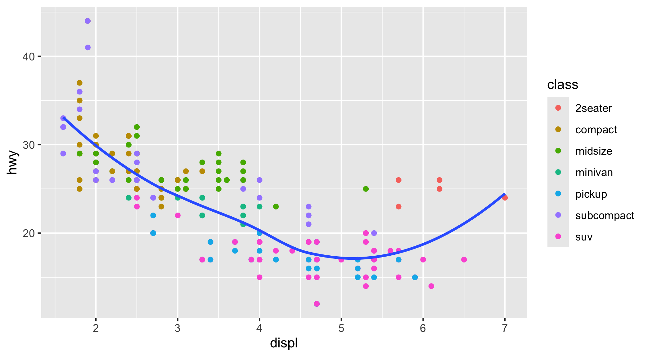
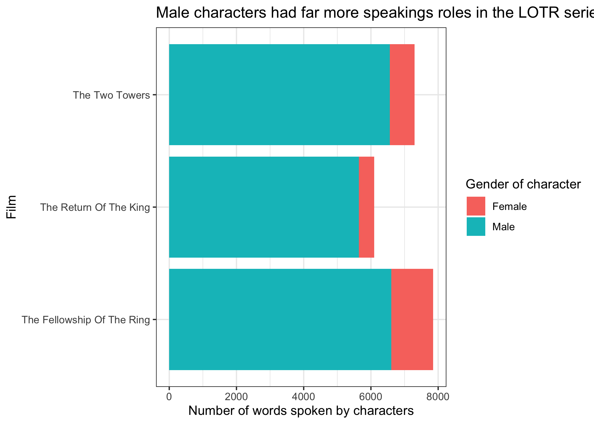
Use the mpg data frame and ggplot to create these charts

Extra practice

Use this link to form teams

Check out some potential project ideas

Week 1: Getting Started

1. Course Goal

2. Course Introduction

3. Quarto

4. Workflow & Reading In Data

5. Wrangling Data

6. Visualizing Data

Week 1: Getting Started

1. Course Goal

2. Course Introduction

3. Quarto

4. Workflow & Reading In Data

5. Wrangling Data

6. Visualizing Data

Course 1: Intro to Programming for Analytics

Class goal: translate data into information

Class goal: translate data into information

Data exploration: an iterative process

Data exploration: an iterative process

Data exploration: an iterative process

A fully reproducible analysis

Data exploration: an iterative process

Week 1: Getting Started

1. Course Goal

2. Course Introduction

3. Quarto

4. Workflow & Reading In Data

5. Wrangling Data

6. Visualizing Data

Meet your instructor!

Meet your tutor!

Prerequisites

EMSE 4574 / 6574: Intro to Programming for Analytics

Course website

Everything you need will be on the course website:https://eda.seas.gwu.edu/2026-Fall/

Quizzes (10% of grade)

At the start of class every other week-ish. Make ups only for excused absences (i.e. don’t be late).

5 total, lowest dropped

10 minutes

Assignments

Grades

Grades

Course policies

Use of AI

We will heavily use AI tools this semester

Ways to not have your work suck:

Late submissions

- 3 late days - use them anytime, no questions asked

- No more than 2 late days on any one assignment

- Contact me for special cases

How to succeed in this class

Getting Help

Course Software

Slack: turn notifications on!

R & Positron (Install both)

Posit Cloud (Register for free!)

Quarto

GitHub Desktop

Break

1. Install everything on the software page

2. Add your GitHub username (NOT GW netID) in this sheet next to your name

Week 1: Getting Started

1. Course Goal

2. Course Introduction

3. Quarto

4. Workflow & Reading In Data

5. Wrangling Data

6. Visualizing Data

This semester we use Positron

(not RStudio)

Positron Orientation

Quick demo

1. Open quarto_demo.qmd

2. Click “Preview”

Anatomy of a .qmd file

Header

Markdown text

R code

Define overall document options in header

Render to multiple outputs

Everything you need will be on the course website:
https://eda.seas.gwu.edu/2026-Fall/

2. Add your GitHub username (NOT GW netID) in
this sheet next to your name

1. Open `quarto_demo.qmd`

A global `setup` chunk 🌍

The tidyverse: `stringr` + `dplyr` + `readr` + `ggplot2` + …

The main `dplyr` “verbs”

Core `tidyverse` concept:
Chain functions together with “pipes”

`%>%`

Select columns with `select()`

Select columns with `select()`

Select columns with `select()`

Filter for rows with `filter()`

Filter for rows with `filter()`

Filter for rows with `filter()`

Filter for rows with `filter()`

Logic operators for `filter()`

Combine `filter()` and `select()`

Create new variables with `mutate()`

Create new variables with `mutate()`

`ifelse(<condition>, <if TRUE>, <else>)`

Sort data frame with `arrange()`

Sort data frame with `arrange()`