Joins & Data Cleaning

EMSE 4572/6572: Exploratory Data Analysis

John Paul Helveston

September 23, 2026

Tip of the week

Copy-paste magic with datapasta

Useful for “small data”: e.g., U.S. State Abbreviations

Today’s data

“Clean” data

wildlife_impacts <- read_csv(file.path('data', 'wildlife_impacts.csv'))
milk_production <- read_csv(file.path('data', 'milk_production.csv'))
msleep <- read_csv(file.path('data', 'msleep.csv'))

“Messy” data

wind <- read_excel(file.path('data', 'US_State_Wind_Energy_Facts_2018.xlsx'))
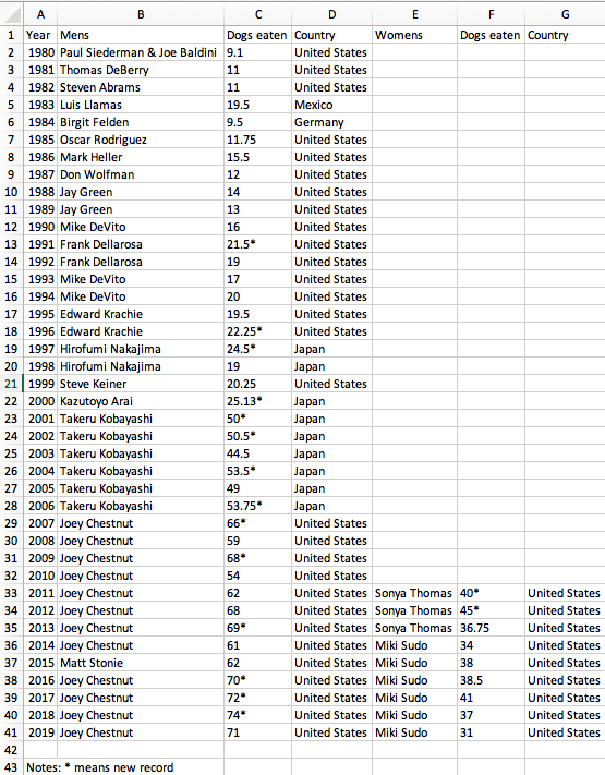
hot_dogs <- read_excel(file.path('data', 'hot_dog_winners.xlsx'))

Plus two new packages:

# For manipulating dates
install.packages('lubridate')

# For cleaning column names
install.packages('janitor')

Week 5: Joins & Data Cleaning

1. Merging datasets with joins

2. Are your variables the right type?

3. Are your variables the right name?

4. Re-coding variables

5. Dates

6. Dealing with messy Excel files

Week 5: Joins & Data Cleaning

1. Merging datasets with joins

2. Are your variables the right type?

3. Are your variables the right name?

4. Re-coding variables

5. Dates

6. Dealing with messy Excel files

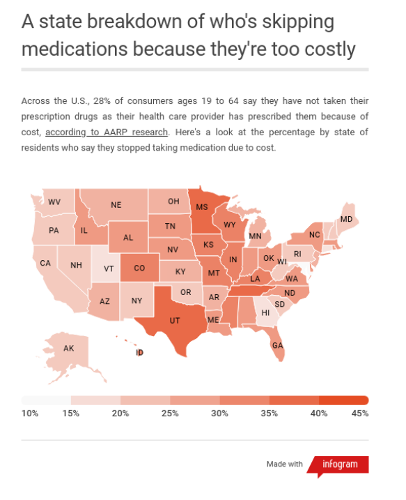
What’s wrong with this map?

Likely culprit: Merging two columns

head(names)

#>   state_name
#> 1    Alabama
#> 2     Alaska
#> 3    Arizona
#> 4   Arkansas
#> 5 California
#> 6   Colorado

head(abbs)

#>   state_abb
#> 1        AK
#> 2        AL
#> 3        AR
#> 4        AZ
#> 5        CA
#> 6        CO

result <- bind_cols(names, abbs)
head(result)

#>   state_name state_abb
#> 1    Alabama        AK
#> 2     Alaska        AL
#> 3    Arizona        AR
#> 4   Arkansas        AZ
#> 5 California        CA
#> 6   Colorado        CO

Joins

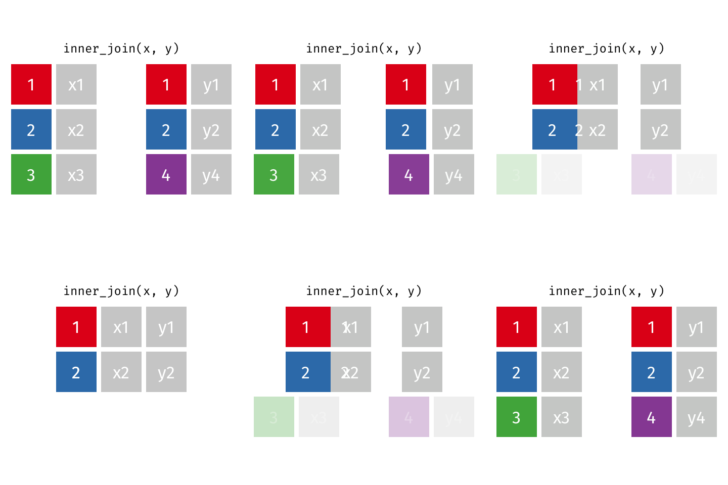
1. inner_join()
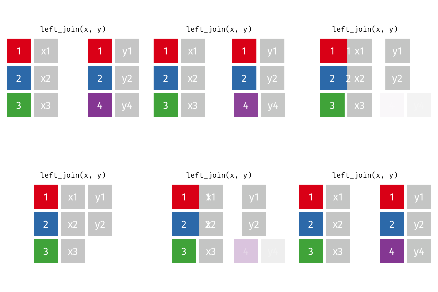
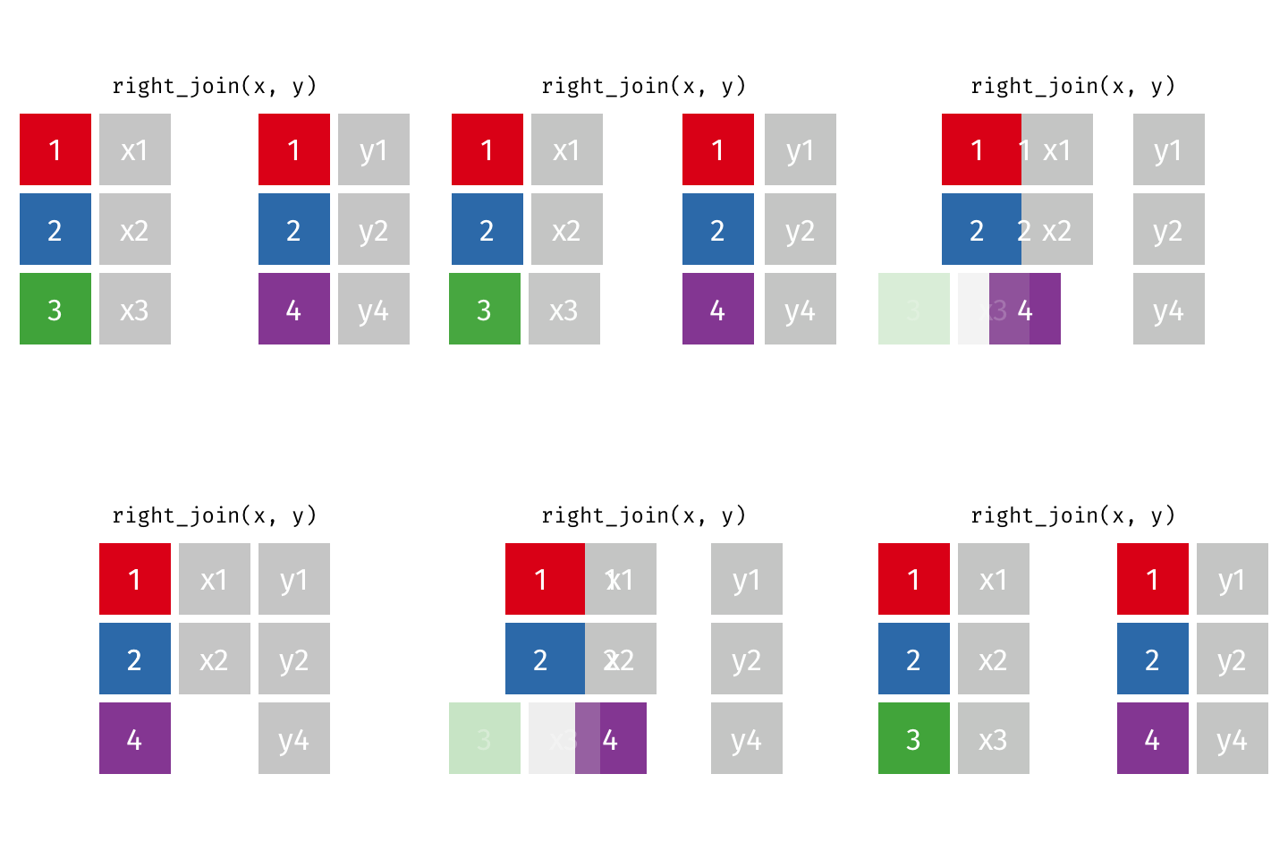
2. left_join() / right_join()
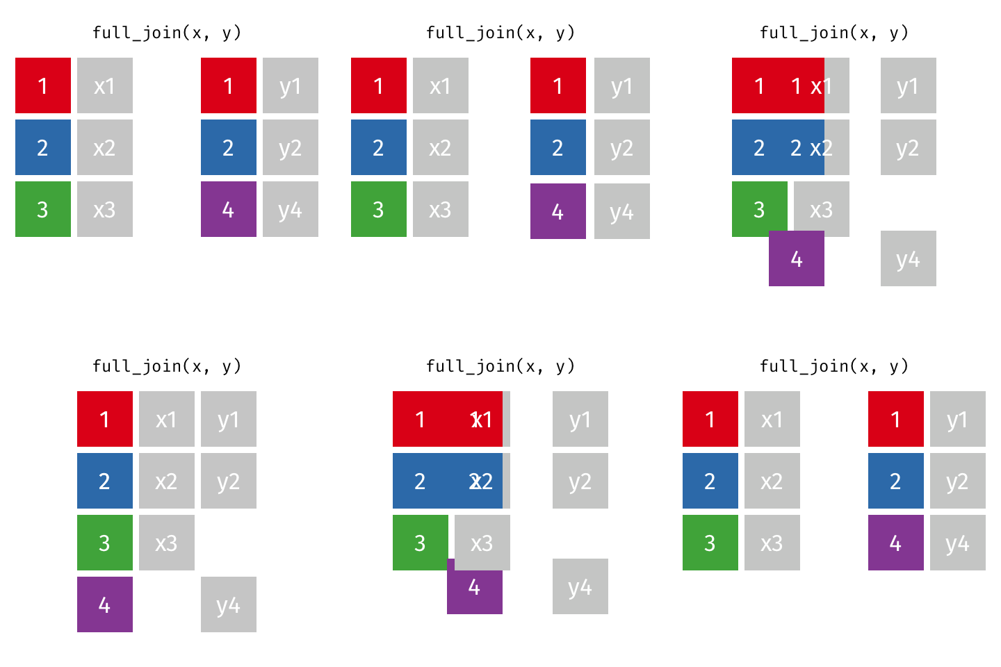
3. full_join()

Example: band_members & band_instruments

band_members

#> # A tibble: 3 × 2
#>   name  band   
#>   <chr> <chr>  
#> 1 Mick  Stones 
#> 2 John  Beatles
#> 3 Paul  Beatles

band_instruments

#> # A tibble: 3 × 2
#>   name  plays 
#>   <chr> <chr> 
#> 1 John  guitar
#> 2 Paul  bass  
#> 3 Keith guitar

inner_join()

band_members %>%
  inner_join(band_instruments)

#> # A tibble: 2 × 3
#>   name  band    plays 
#>   <chr> <chr>   <chr> 
#> 1 John  Beatles guitar
#> 2 Paul  Beatles bass

full_join()

band_members %>%
  full_join(band_instruments)

#> # A tibble: 4 × 3
#>   name  band    plays 
#>   <chr> <chr>   <chr> 
#> 1 Mick  Stones  <NA>  
#> 2 John  Beatles guitar
#> 3 Paul  Beatles bass  
#> 4 Keith <NA>    guitar

left_join()

band_members %>%
  left_join(band_instruments)

#> # A tibble: 3 × 3
#>   name  band    plays 
#>   <chr> <chr>   <chr> 
#> 1 Mick  Stones  <NA>  
#> 2 John  Beatles guitar
#> 3 Paul  Beatles bass

right_join()

band_members %>%
  right_join(band_instruments)

#> # A tibble: 3 × 3
#>   name  band    plays 
#>   <chr> <chr>   <chr> 
#> 1 John  Beatles guitar
#> 2 Paul  Beatles bass  
#> 3 Keith <NA>    guitar

Specify the joining variable name

band_members %>%
  left_join(band_instruments)

#> Joining with `by = join_by(name)`

#> # A tibble: 3 × 3
#>   name  band    plays 
#>   <chr> <chr>   <chr> 
#> 1 Mick  Stones  <NA>  
#> 2 John  Beatles guitar
#> 3 Paul  Beatles bass

band_members %>%
  left_join(
    band_instruments,
    by = 'name'
  )

#> # A tibble: 3 × 3
#>   name  band    plays 
#>   <chr> <chr>   <chr> 
#> 1 Mick  Stones  <NA>  
#> 2 John  Beatles guitar
#> 3 Paul  Beatles bass

Specify the joining variable name

If the names differ, use by = c("left_name" = "joining_name")

band_members

#> # A tibble: 3 × 2
#>   name  band   
#>   <chr> <chr>  
#> 1 Mick  Stones 
#> 2 John  Beatles
#> 3 Paul  Beatles

band_instruments2

#> # A tibble: 3 × 2
#>   artist plays 
#>   <chr>  <chr> 
#> 1 John   guitar
#> 2 Paul   bass  
#> 3 Keith  guitar

band_members %>%
  left_join(
    band_instruments2,
    by = c("name" = "artist")
  )

#> # A tibble: 3 × 3
#>   name  band    plays 
#>   <chr> <chr>   <chr> 
#> 1 Mick  Stones  <NA>  
#> 2 John  Beatles guitar
#> 3 Paul  Beatles bass

Specify the joining variable name

Or just rename the joining variable in a pipe

band_members

#> # A tibble: 3 × 2
#>   name  band   
#>   <chr> <chr>  
#> 1 Mick  Stones 
#> 2 John  Beatles
#> 3 Paul  Beatles

band_instruments2

#> # A tibble: 3 × 2
#>   artist plays 
#>   <chr>  <chr> 
#> 1 John   guitar
#> 2 Paul   bass  
#> 3 Keith  guitar

band_members %>%
  rename(artist = name) %>%
  left_join(
    band_instruments2,
    by = "artist"
  )

#> # A tibble: 3 × 3
#>   artist band    plays 
#>   <chr>  <chr>   <chr> 
#> 1 Mick   Stones  <NA>  
#> 2 John   Beatles guitar
#> 3 Paul   Beatles bass

15:00

Your turn

1. Create a data frame called state_data by joining the data frames states_abbs and milk_production and then selecting the variables region, state_name, state_abb. Hint: Use the distinct() function to drop repeated rows.

Your result should look like this:

head(state_data)

#> # A tibble: 6 × 3
#>   region    state_name    state_abb
#>   <chr>     <chr>         <chr>    
#> 1 Northeast Maine         ME       
#> 2 Northeast New Hampshire NH       
#> 3 Northeast Vermont       VT       
#> 4 Northeast Massachusetts MA       
#> 5 Northeast Rhode Island  RI       
#> 6 Northeast Connecticut   CT

2. Join the state_data data frame to the wildlife_impacts data frame, adding the variables region and state_name

glimpse(wildlife_impacts)

#> Rows: 56,978
#> Columns: 24
#> $ region                <chr> "Northeast", "Northeast", "Northeast", "Northeast", "Northeast", "Northeast", "Northeast", "Northeast", "Northeast", "Northeast", "Northeast", "Northeast", "Northeast", "Northeast", "Northeast", "Northeast", "Northeast…
#> $ state_name            <chr> "Maine", "Maine", "Maine", "Maine", "Maine", "Maine", "Maine", "Maine", "Maine", "Maine", "Maine", "Maine", "Maine", "Maine", "Maine", "Maine", "Maine", "Maine", "Maine", "Maine", "Maine", "Maine", "Maine", "Maine", "M…
#> $ state_abb             <chr> "ME", "ME", "ME", "ME", "ME", "ME", "ME", "ME", "ME", "ME", "ME", "ME", "ME", "ME", "ME", "ME", "ME", "ME", "ME", "ME", "ME", "ME", "ME", "ME", "ME", "ME", "ME", "ME", "ME", "ME", "ME", "ME", "ME", "ME", "ME", "ME", "M…
#> $ incident_date         <dttm> 2018-10-23, 2018-10-07, 2018-10-05, 2018-10-05, 2017-07-25, 2016-11-07, 2016-11-07, 2016-10-29, 2016-07-30, 1990-08-01, 2018-11-06, 2018-07-29, 2018-05-05, 2017-04-04, 2016-04-28, 2012-05-20, 2011-10-23, 2003-09-07, 2…
#> $ airport_id            <chr> "KPWM", "KPWM", "KPWM", "KPWM", "KPWM", "KPWM", "KPWM", "KPWM", "KPWM", "KPWM", "KPWM", "KPWM", "KPWM", "KPWM", "KPWM", "KPWM", "KPWM", "KPWM", "KPWM", "KPWM", "KPWM", "KBGR", "KPWM", "KBGR", "KPWM", "KPWM", "KPWM", "K…
#> $ airport               <chr> "PORTLAND INTL JETPORT (ME)", "PORTLAND INTL JETPORT (ME)", "PORTLAND INTL JETPORT (ME)", "PORTLAND INTL JETPORT (ME)", "PORTLAND INTL JETPORT (ME)", "PORTLAND INTL JETPORT (ME)", "PORTLAND INTL JETPORT (ME)", "PORTLAN…
#> $ operator              <chr> "AMERICAN AIRLINES", "AMERICAN AIRLINES", "AMERICAN AIRLINES", "AMERICAN AIRLINES", "AMERICAN AIRLINES", "AMERICAN AIRLINES", "AMERICAN AIRLINES", "AMERICAN AIRLINES", "AMERICAN AIRLINES", "AMERICAN AIRLINES", "DELTA A…
#> $ atype                 <chr> "A-320", "A-319", "A-319", "EMB-190", "EMB-170", "A-319", "A-319", "A-319", "CRJ100/200", "DHC8 DASH 8", "MD-90-30", "MD-90-30", "MD-90-30", "CRJ700", "MD-88", "MD-88", "MD-88", "MD-88", "MD-88", "MD-80", "MD-88", "MD-…
#> $ type_eng              <chr> "D", "D", "D", "D", "D", "D", "D", "D", "D", "C", "D", "D", "D", "D", "D", "D", "D", "D", "D", "D", "D", "D", "D", "D", "D", "D", "D", "D", "D", "D", "D", "D", "D", "D", "D", "D", "D", "D", "D", "D", "D", "D", "D", "D"…
#> $ species_id            <chr> "UNKBS", "ZX302", "ZS010", "I1102", "K3310", "YH004", "UNKB", "YL001", "UNKB", "NE1", "R2001", "YM1102", "NE101", "YL001", "UNKB", "NE1", "UNKB", "I1102", "UNKBS", "NE1", "NE101", "ZX202", "ZX3", "ZX202", "NE1", "UNKBS…
#> $ species               <chr> "Unknown bird - small", "Swamp sparrow", "Blackpoll warbler", "Great blue heron", "Sharp-shinned hawk", "Horned lark", "Unknown bird", "European starling", "Unknown bird", "Gulls", "Snowy owl", "American crow", "Herrin…
#> $ damage                <chr> "N", NA, "N", "M?", "N", "N", "N", "N", "N", "N", NA, "N", "N", NA, "N", NA, "N", NA, NA, "N", "M", "N", "N", "N", "N", "N", "N", "N", "N", "N", NA, "N", "N", "N", "N", "N", "N", "N", "N", "N", "N", "N", "N", "N", "N",…
#> $ num_engs              <dbl> 2, 2, 2, 2, 2, 2, 2, 2, 2, 2, 2, 2, 2, 2, 2, 2, 2, 2, 2, 2, 2, 2, 2, 2, 2, 2, 3, 2, 2, 2, 2, 2, 2, 2, 2, 2, 2, 2, 2, 2, 2, 2, 2, 2, 2, 2, 2, 2, 2, 2, 3, 3, 3, 3, 2, 2, 3, 3, 2, 2, 2, 2, 2, 2, 2, 2, 2, 2, 2, 2, 2, 2, 2,…
#> $ incident_month        <dbl> 10, 10, 10, 10, 7, 11, 11, 10, 7, 8, 11, 7, 5, 4, 4, 5, 10, 9, 8, 6, 6, 11, 11, 11, 10, 5, 10, 8, 11, 9, 11, 10, 11, 11, 10, 10, 10, 9, 11, 7, 6, 6, 6, 6, 9, 8, 6, 5, 11, 7, 8, 9, 5, 5, 10, 2, 9, 8, 3, 3, 3, 11, 11, 11…
#> $ incident_year         <dbl> 2018, 2018, 2018, 2018, 2017, 2016, 2016, 2016, 2016, 1990, 2018, 2018, 2018, 2017, 2016, 2012, 2011, 2003, 2002, 2000, 2000, 1995, 1995, 1995, 1995, 1995, 1994, 1994, 1993, 1993, 1992, 1990, 2018, 2018, 2018, 2018, 20…
#> $ time_of_day           <chr> NA, "Night", "Night", "Day", "Dawn", "Day", "Day", "Day", "Day", "Day", "Dawn", "Day", "Day", NA, "Night", "Day", NA, "Night", "Day", "Day", "Day", "Day", "Day", "Dawn", "Day", "Day", "Night", "Day", "Day", "Night", "N…
#> $ time                  <dbl> 1310, 1035, 2200, 1645, 645, 1345, 1346, 1400, 1100, NA, 610, 1912, 613, 1145, 2041, 700, NA, 2035, NA, NA, NA, NA, NA, NA, NA, NA, NA, NA, NA, NA, NA, NA, 1515, 1545, 1523, 1610, 1025, 2343, 1533, 1115, 1145, 1130, 11…
#> $ height                <dbl> 15, NA, 1000, 0, 0, 0, 0, NA, NA, 2000, 0, 50, 0, 0, NA, 0, 0, 0, 0, 200, 0, 0, 10, 0, 0, 0, 2500, 0, 3, 200, 0, 0, 5, 20, 0, 10, 0, 800, 0, 50, 0, 0, NA, 1300, 2000, 30, 0, 1300, 2000, 1500, 500, NA, NA, NA, 0, 0, 0, …
#> $ speed                 <dbl> 150, NA, 140, 110, NA, NA, NA, NA, NA, 250, 100, NA, 150, NA, NA, NA, NA, 130, 130, 135, NA, 85, 140, 150, NA, 125, 140, NA, 135, 120, 90, NA, 131, 140, NA, 155, NA, NA, NA, 140, NA, 100, NA, 150, 150, 140, NA, 150, 21…
#> $ phase_of_flt          <chr> "departure", "arrival", "arrival", "arrival", "arrival", "arrival", "arrival", "arrival", "arrival", "departure", "departure", "departure", "departure", "arrival", "arrival", "departure", "arrival", "arrival", "departu…
#> $ sky                   <chr> "Overcast", "Some Cloud", "Some Cloud", "Some Cloud", "Some Cloud", "No Cloud", NA, "Overcast", "Overcast", NA, "Overcast", "Some Cloud", "Some Cloud", "Overcast", NA, "No Cloud", NA, "Overcast", "Overcast", "Overcast"…
#> $ precip                <chr> "None", "None", "None", "None", "None", "None", NA, "Rain", "None", NA, "Rain", "None", "None", "Rain", NA, "None", NA, NA, "None", "None", "None", "None", "None", "None", "None", "None", "Rain", "None", "None", "None"…
#> $ cost_repairs_infl_adj <dbl> NA, NA, NA, NA, NA, NA, NA, NA, NA, NA, NA, NA, NA, NA, NA, NA, NA, NA, NA, NA, NA, NA, NA, NA, NA, NA, NA, NA, NA, NA, NA, NA, NA, 5400, NA, NA, NA, NA, NA, NA, NA, NA, NA, NA, NA, NA, NA, NA, NA, NA, NA, NA, NA, NA, …
#> $ weekday_name          <ord> Tue, Sun, Fri, Fri, Tue, Mon, Mon, Sat, Sat, Wed, Tue, Sun, Sat, Tue, Thu, Sun, Sun, Sun, Fri, Tue, Tue, Tue, Mon, Sat, Tue, Mon, Sat, Tue, Thu, Sat, Tue, Fri, Fri, Sat, Tue, Sat, Wed, Tue, Thu, Thu, Sun, Sun, Sun, Fri…

Week 5: Joins & Data Cleaning

1. Merging datasets with joins

2. Are your variables the right type?

3. Are your variables the right name?

4. Re-coding variables

5. Dates

6. Dealing with messy Excel files

Always check variable types after reading in data!

wind <- read_excel(file.path(
  'data',
  'US_State_Wind_Energy_Facts_2018.xlsx'
))

glimpse(wind)

#> Rows: 50
#> Columns: 7
#> $ Ranking                         <chr> "1.0", "2.0", "3.0", "4.0", "5.0", "6.0", "7.0", "8.0", "9.0", "10.0", "11.0", "12.0", "13.0", "14.0", "15.0", "16.0", "17.0", "18.0", "19.0", "20.0", "21.0", "22.0", "23.0", "24.0", "25.0", "26.0", "27.0", "…
#> $ State                           <chr> "TEXAS", "OKLAHOMA", "IOWA", "CALIFORNIA", "KANSAS", "ILLINOIS", "MINNESOTA", "OREGON", "COLORADO", "WASHINGTON", "NORTH DAKOTA", "INDIANA", "MICHIGAN", "NEW YORK", "NEW MEXICO", "WYOMING", "NEBRASKA", "PENNS…
#> $ `Installed Capacity (MW)`       <dbl> 23262, 7495, 7312, 5686, 5110, 4464, 3699, 3213, 3106, 3075, 2996, 2117, 1904, 1829, 1682, 1489, 1445, 1369, 977, 973, 959, 923, 746, 720, 686, 617, 391, 268, 208, 206, 191, 185, 152, 149, 113, 62, 54, 29, 9,…
#> $ `Equivalent Homes Powered`      <chr> "6235000.0", "2268000.0", "1935000.0", "1298000.0", "1719000.0", "1050000.0", "1012000.0", "604600.0", "889100.0", "695300.0", "1021000.0", "440700.0", "471700.0", "366500.0", "422100.0", "408700.0", "486700.…
#> $ `Total Investment ($ Millions)` <chr> "42000.0", "13700.0", "14200.0", "12600.0", "9400.0", "8900.0", "7100.0", "6600.0", "6000.0", "6100.0", "5800.0", "4500.0", "3500.0", "3700.0", "2900.0", "3100.0", "2600.0", "2800.0", "2100.0", "2100.0", "180…
#> $ `Wind Projects Online`          <dbl> 136, 45, 107, 104, 35, 49, 98, 31, 25, 20, 28, 16, 26, 27, 17, 22, 22, 24, 14, 15, 8, 18, 18, 16, 6, 37, 5, 5, 1, 7, 6, 5, 1, 9, 44, 19, 15, 2, 2, 2, 1, 0, 1, 0, 0, 0, 0, 0, 0, 0
#> $ `# of Wind Turbines`            <chr> "12750.0", "3717.0", "4145.0", "6972.0", "2795.0", "2632.0", "2428.0", "1868.0", "1949.0", "1725.0", "1611.0", "1203.0", "1051.0", "1052.0", "1005.0", "1005.0", "789.0", "726.0", "583.0", "541.0", "499.0", "3…

Be careful converting strings to numbers!

as.numeric()

as.numeric(c("2.1", "3.7", "4.50"))

#> [1] 2.1 3.7 4.5

as.numeric(c("$2.1", "$3.7", "$4.50"))

#> [1] NA NA NA

parse_number()

parse_number(c("2.1", "3.7", "4.50"))

#> [1] 2.1 3.7 4.5

parse_number(c("$2.1", "$3.7", "$4.50"))

#> [1] 2.1 3.7 4.5

parse_number(c("1-800-123-4567"))

#> [1] 1

Week 5: Joins & Data Cleaning

1. Merging datasets with joins

2. Are your variables the right type?

3. Are your variables the right name?

4. Re-coding variables

5. Dates

6. Dealing with messy Excel files

Renaming made easy

janitor::clean_names()

wind <- read_excel(file.path(
  'data',
  'US_State_Wind_Energy_Facts_2018.xlsx'
))

glimpse(wind)

#> Rows: 50
#> Columns: 7
#> $ Ranking                         <chr> "1.0", "2.0", "3.0", "4.0", "5.0", "6.0", "7.0", "8.0", "9.0", "10.0", "11.0", "12.0", "13.0", "14.0", "15.0", "16.0", "17.0", "18.0", "19.0", "20.0", "21.0", "22.0", "23.0", "24.0", "25.0", "26.0", "27.0", "…
#> $ State                           <chr> "TEXAS", "OKLAHOMA", "IOWA", "CALIFORNIA", "KANSAS", "ILLINOIS", "MINNESOTA", "OREGON", "COLORADO", "WASHINGTON", "NORTH DAKOTA", "INDIANA", "MICHIGAN", "NEW YORK", "NEW MEXICO", "WYOMING", "NEBRASKA", "PENNS…
#> $ `Installed Capacity (MW)`       <dbl> 23262, 7495, 7312, 5686, 5110, 4464, 3699, 3213, 3106, 3075, 2996, 2117, 1904, 1829, 1682, 1489, 1445, 1369, 977, 973, 959, 923, 746, 720, 686, 617, 391, 268, 208, 206, 191, 185, 152, 149, 113, 62, 54, 29, 9,…
#> $ `Equivalent Homes Powered`      <chr> "6235000.0", "2268000.0", "1935000.0", "1298000.0", "1719000.0", "1050000.0", "1012000.0", "604600.0", "889100.0", "695300.0", "1021000.0", "440700.0", "471700.0", "366500.0", "422100.0", "408700.0", "486700.…
#> $ `Total Investment ($ Millions)` <chr> "42000.0", "13700.0", "14200.0", "12600.0", "9400.0", "8900.0", "7100.0", "6600.0", "6000.0", "6100.0", "5800.0", "4500.0", "3500.0", "3700.0", "2900.0", "3100.0", "2600.0", "2800.0", "2100.0", "2100.0", "180…
#> $ `Wind Projects Online`          <dbl> 136, 45, 107, 104, 35, 49, 98, 31, 25, 20, 28, 16, 26, 27, 17, 22, 22, 24, 14, 15, 8, 18, 18, 16, 6, 37, 5, 5, 1, 7, 6, 5, 1, 9, 44, 19, 15, 2, 2, 2, 1, 0, 1, 0, 0, 0, 0, 0, 0, 0
#> $ `# of Wind Turbines`            <chr> "12750.0", "3717.0", "4145.0", "6972.0", "2795.0", "2632.0", "2428.0", "1868.0", "1949.0", "1725.0", "1611.0", "1203.0", "1051.0", "1052.0", "1005.0", "1005.0", "789.0", "726.0", "583.0", "541.0", "499.0", "3…

Renaming made easy

janitor::clean_names()

library(janitor)

wind <- read_excel(file.path(
  'data',
  'US_State_Wind_Energy_Facts_2018.xlsx'
)) %>%
  clean_names()

glimpse(wind)

#> Rows: 50
#> Columns: 7
#> $ ranking                   <chr> "1.0", "2.0", "3.0", "4.0", "5.0", "6.0", "7.0", "8.0", "9.0", "10.0", "11.0", "12.0", "13.0", "14.0", "15.0", "16.0", "17.0", "18.0", "19.0", "20.0", "21.0", "22.0", "23.0", "24.0", "25.0", "26.0", "27.0", "28.0",…
#> $ state                     <chr> "TEXAS", "OKLAHOMA", "IOWA", "CALIFORNIA", "KANSAS", "ILLINOIS", "MINNESOTA", "OREGON", "COLORADO", "WASHINGTON", "NORTH DAKOTA", "INDIANA", "MICHIGAN", "NEW YORK", "NEW MEXICO", "WYOMING", "NEBRASKA", "PENNSYLVANI…
#> $ installed_capacity_mw     <dbl> 23262, 7495, 7312, 5686, 5110, 4464, 3699, 3213, 3106, 3075, 2996, 2117, 1904, 1829, 1682, 1489, 1445, 1369, 977, 973, 959, 923, 746, 720, 686, 617, 391, 268, 208, 206, 191, 185, 152, 149, 113, 62, 54, 29, 9, 5, 2,…
#> $ equivalent_homes_powered  <chr> "6235000.0", "2268000.0", "1935000.0", "1298000.0", "1719000.0", "1050000.0", "1012000.0", "604600.0", "889100.0", "695300.0", "1021000.0", "440700.0", "471700.0", "366500.0", "422100.0", "408700.0", "486700.0", "3…
#> $ total_investment_millions <chr> "42000.0", "13700.0", "14200.0", "12600.0", "9400.0", "8900.0", "7100.0", "6600.0", "6000.0", "6100.0", "5800.0", "4500.0", "3500.0", "3700.0", "2900.0", "3100.0", "2600.0", "2800.0", "2100.0", "2100.0", "1800.0", …
#> $ wind_projects_online      <dbl> 136, 45, 107, 104, 35, 49, 98, 31, 25, 20, 28, 16, 26, 27, 17, 22, 22, 24, 14, 15, 8, 18, 18, 16, 6, 37, 5, 5, 1, 7, 6, 5, 1, 9, 44, 19, 15, 2, 2, 2, 1, 0, 1, 0, 0, 0, 0, 0, 0, 0
#> $ number_of_wind_turbines   <chr> "12750.0", "3717.0", "4145.0", "6972.0", "2795.0", "2632.0", "2428.0", "1868.0", "1949.0", "1725.0", "1611.0", "1203.0", "1051.0", "1052.0", "1005.0", "1005.0", "789.0", "726.0", "583.0", "541.0", "499.0", "386.0",…

Renaming made easy

janitor::clean_names()

library(janitor)

wind <- read_excel(file.path(
  'data',
  'US_State_Wind_Energy_Facts_2018.xlsx'
)) %>%
  clean_names(case = 'lower_camel')

glimpse(wind)

#> Rows: 50
#> Columns: 7
#> $ ranking                 <chr> "1.0", "2.0", "3.0", "4.0", "5.0", "6.0", "7.0", "8.0", "9.0", "10.0", "11.0", "12.0", "13.0", "14.0", "15.0", "16.0", "17.0", "18.0", "19.0", "20.0", "21.0", "22.0", "23.0", "24.0", "25.0", "26.0", "27.0", "28.0", "…
#> $ state                   <chr> "TEXAS", "OKLAHOMA", "IOWA", "CALIFORNIA", "KANSAS", "ILLINOIS", "MINNESOTA", "OREGON", "COLORADO", "WASHINGTON", "NORTH DAKOTA", "INDIANA", "MICHIGAN", "NEW YORK", "NEW MEXICO", "WYOMING", "NEBRASKA", "PENNSYLVANIA"…
#> $ installedCapacityMw     <dbl> 23262, 7495, 7312, 5686, 5110, 4464, 3699, 3213, 3106, 3075, 2996, 2117, 1904, 1829, 1682, 1489, 1445, 1369, 977, 973, 959, 923, 746, 720, 686, 617, 391, 268, 208, 206, 191, 185, 152, 149, 113, 62, 54, 29, 9, 5, 2, 0…
#> $ equivalentHomesPowered  <chr> "6235000.0", "2268000.0", "1935000.0", "1298000.0", "1719000.0", "1050000.0", "1012000.0", "604600.0", "889100.0", "695300.0", "1021000.0", "440700.0", "471700.0", "366500.0", "422100.0", "408700.0", "486700.0", "314…
#> $ totalInvestmentMillions <chr> "42000.0", "13700.0", "14200.0", "12600.0", "9400.0", "8900.0", "7100.0", "6600.0", "6000.0", "6100.0", "5800.0", "4500.0", "3500.0", "3700.0", "2900.0", "3100.0", "2600.0", "2800.0", "2100.0", "2100.0", "1800.0", "1…
#> $ windProjectsOnline      <dbl> 136, 45, 107, 104, 35, 49, 98, 31, 25, 20, 28, 16, 26, 27, 17, 22, 22, 24, 14, 15, 8, 18, 18, 16, 6, 37, 5, 5, 1, 7, 6, 5, 1, 9, 44, 19, 15, 2, 2, 2, 1, 0, 1, 0, 0, 0, 0, 0, 0, 0
#> $ numberOfWindTurbines    <chr> "12750.0", "3717.0", "4145.0", "6972.0", "2795.0", "2632.0", "2428.0", "1868.0", "1949.0", "1725.0", "1611.0", "1203.0", "1051.0", "1052.0", "1005.0", "1005.0", "789.0", "726.0", "583.0", "541.0", "499.0", "386.0", "…

Renaming made easy

janitor::clean_names()

library(janitor)

wind <- read_excel(file.path(
  'data',
  'US_State_Wind_Energy_Facts_2018.xlsx'
)) %>%
  clean_names(case = 'screaming_snake')

glimpse(wind)

#> Rows: 50
#> Columns: 7
#> $ RANKING                   <chr> "1.0", "2.0", "3.0", "4.0", "5.0", "6.0", "7.0", "8.0", "9.0", "10.0", "11.0", "12.0", "13.0", "14.0", "15.0", "16.0", "17.0", "18.0", "19.0", "20.0", "21.0", "22.0", "23.0", "24.0", "25.0", "26.0", "27.0", "28.0",…
#> $ STATE                     <chr> "TEXAS", "OKLAHOMA", "IOWA", "CALIFORNIA", "KANSAS", "ILLINOIS", "MINNESOTA", "OREGON", "COLORADO", "WASHINGTON", "NORTH DAKOTA", "INDIANA", "MICHIGAN", "NEW YORK", "NEW MEXICO", "WYOMING", "NEBRASKA", "PENNSYLVANI…
#> $ INSTALLED_CAPACITY_MW     <dbl> 23262, 7495, 7312, 5686, 5110, 4464, 3699, 3213, 3106, 3075, 2996, 2117, 1904, 1829, 1682, 1489, 1445, 1369, 977, 973, 959, 923, 746, 720, 686, 617, 391, 268, 208, 206, 191, 185, 152, 149, 113, 62, 54, 29, 9, 5, 2,…
#> $ EQUIVALENT_HOMES_POWERED  <chr> "6235000.0", "2268000.0", "1935000.0", "1298000.0", "1719000.0", "1050000.0", "1012000.0", "604600.0", "889100.0", "695300.0", "1021000.0", "440700.0", "471700.0", "366500.0", "422100.0", "408700.0", "486700.0", "3…
#> $ TOTAL_INVESTMENT_MILLIONS <chr> "42000.0", "13700.0", "14200.0", "12600.0", "9400.0", "8900.0", "7100.0", "6600.0", "6000.0", "6100.0", "5800.0", "4500.0", "3500.0", "3700.0", "2900.0", "3100.0", "2600.0", "2800.0", "2100.0", "2100.0", "1800.0", …
#> $ WIND_PROJECTS_ONLINE      <dbl> 136, 45, 107, 104, 35, 49, 98, 31, 25, 20, 28, 16, 26, 27, 17, 22, 22, 24, 14, 15, 8, 18, 18, 16, 6, 37, 5, 5, 1, 7, 6, 5, 1, 9, 44, 19, 15, 2, 2, 2, 1, 0, 1, 0, 0, 0, 0, 0, 0, 0
#> $ NUMBER_OF_WIND_TURBINES   <chr> "12750.0", "3717.0", "4145.0", "6972.0", "2795.0", "2632.0", "2428.0", "1868.0", "1949.0", "1725.0", "1611.0", "1203.0", "1051.0", "1052.0", "1005.0", "1005.0", "789.0", "726.0", "583.0", "541.0", "499.0", "386.0",…

select(): more powerful than you probably thought

Example: data on sleeping patterns of different mammals

glimpse(msleep)

#> Rows: 83
#> Columns: 11
#> $ name         <chr> "Cheetah", "Owl monkey", "Mountain beaver", "Greater short-tailed shrew", "Cow", "Three-toed sloth", "Northern fur seal", "Vesper mouse", "Dog", "Roe deer", "Goat", "Guinea pig", "Grivet", "Chinchilla", "Star-nosed mole", "Afri…
#> $ genus        <chr> "Acinonyx", "Aotus", "Aplodontia", "Blarina", "Bos", "Bradypus", "Callorhinus", "Calomys", "Canis", "Capreolus", "Capri", "Cavis", "Cercopithecus", "Chinchilla", "Condylura", "Cricetomys", "Cryptotis", "Dasypus", "Dendrohyrax",…
#> $ vore         <chr> "carni", "omni", "herbi", "omni", "herbi", "herbi", "carni", NA, "carni", "herbi", "herbi", "herbi", "omni", "herbi", "omni", "omni", "omni", "carni", "herbi", "omni", "herbi", "insecti", "herbi", "herbi", "omni", "omni", "herb…
#> $ order        <chr> "Carnivora", "Primates", "Rodentia", "Soricomorpha", "Artiodactyla", "Pilosa", "Carnivora", "Rodentia", "Carnivora", "Artiodactyla", "Artiodactyla", "Rodentia", "Primates", "Rodentia", "Soricomorpha", "Rodentia", "Soricomorpha"…
#> $ conservation <chr> "lc", NA, "nt", "lc", "domesticated", NA, "vu", NA, "domesticated", "lc", "lc", "domesticated", "lc", "domesticated", "lc", NA, "lc", "lc", "lc", "lc", "en", "lc", "domesticated", "domesticated", "lc", "lc", NA, "domesticated",…
#> $ sleep_total  <dbl> 12.1, 17.0, 14.4, 14.9, 4.0, 14.4, 8.7, 7.0, 10.1, 3.0, 5.3, 9.4, 10.0, 12.5, 10.3, 8.3, 9.1, 17.4, 5.3, 18.0, 3.9, 19.7, 2.9, 3.1, 10.1, 10.9, 14.9, 12.5, 9.8, 1.9, 2.7, 6.2, 6.3, 8.0, 9.5, 3.3, 19.4, 10.1, 14.2, 14.3, 12.8, 1…
#> $ sleep_rem    <dbl> NA, 1.8, 2.4, 2.3, 0.7, 2.2, 1.4, NA, 2.9, NA, 0.6, 0.8, 0.7, 1.5, 2.2, 2.0, 1.4, 3.1, 0.5, 4.9, NA, 3.9, 0.6, 0.4, 3.5, 1.1, NA, 3.2, 1.1, 0.4, 0.1, 1.5, 0.6, 1.9, 0.9, NA, 6.6, 1.2, 1.9, 3.1, NA, 1.4, 2.0, NA, NA, 0.9, NA, 0.…
#> $ sleep_cycle  <dbl> NA, NA, NA, 0.1333333, 0.6666667, 0.7666667, 0.3833333, NA, 0.3333333, NA, NA, 0.2166667, NA, 0.1166667, NA, NA, 0.1500000, 0.3833333, NA, 0.3333333, NA, 0.1166667, 1.0000000, NA, 0.2833333, NA, NA, 0.4166667, 0.5500000, NA, NA…
#> $ awake        <dbl> 11.90, 7.00, 9.60, 9.10, 20.00, 9.60, 15.30, 17.00, 13.90, 21.00, 18.70, 14.60, 14.00, 11.50, 13.70, 15.70, 14.90, 6.60, 18.70, 6.00, 20.10, 4.30, 21.10, 20.90, 13.90, 13.10, 9.10, 11.50, 14.20, 22.10, 21.35, 17.80, 17.70, 16.0…
#> $ brainwt      <dbl> NA, 0.01550, NA, 0.00029, 0.42300, NA, NA, NA, 0.07000, 0.09820, 0.11500, 0.00550, NA, 0.00640, 0.00100, 0.00660, 0.00014, 0.01080, 0.01230, 0.00630, 4.60300, 0.00030, 0.65500, 0.41900, 0.00350, 0.11500, NA, 0.02560, 0.00500, N…
#> $ bodywt       <dbl> 50.000, 0.480, 1.350, 0.019, 600.000, 3.850, 20.490, 0.045, 14.000, 14.800, 33.500, 0.728, 4.750, 0.420, 0.060, 1.000, 0.005, 3.500, 2.950, 1.700, 2547.000, 0.023, 521.000, 187.000, 0.770, 10.000, 0.071, 3.300, 0.200, 899.995, …

select(): more powerful than you probably thought

Use select() to choose which columns to keep

msleep %>%
  select(name:order, sleep_total:sleep_cycle) %>%
  glimpse()

#> Rows: 83
#> Columns: 7
#> $ name        <chr> "Cheetah", "Owl monkey", "Mountain beaver", "Greater short-tailed shrew", "Cow", "Three-toed sloth", "Northern fur seal", "Vesper mouse", "Dog", "Roe deer", "Goat", "Guinea pig", "Grivet", "Chinchilla", "Star-nosed mole", "Afric…
#> $ genus       <chr> "Acinonyx", "Aotus", "Aplodontia", "Blarina", "Bos", "Bradypus", "Callorhinus", "Calomys", "Canis", "Capreolus", "Capri", "Cavis", "Cercopithecus", "Chinchilla", "Condylura", "Cricetomys", "Cryptotis", "Dasypus", "Dendrohyrax", …
#> $ vore        <chr> "carni", "omni", "herbi", "omni", "herbi", "herbi", "carni", NA, "carni", "herbi", "herbi", "herbi", "omni", "herbi", "omni", "omni", "omni", "carni", "herbi", "omni", "herbi", "insecti", "herbi", "herbi", "omni", "omni", "herbi…
#> $ order       <chr> "Carnivora", "Primates", "Rodentia", "Soricomorpha", "Artiodactyla", "Pilosa", "Carnivora", "Rodentia", "Carnivora", "Artiodactyla", "Artiodactyla", "Rodentia", "Primates", "Rodentia", "Soricomorpha", "Rodentia", "Soricomorpha",…
#> $ sleep_total <dbl> 12.1, 17.0, 14.4, 14.9, 4.0, 14.4, 8.7, 7.0, 10.1, 3.0, 5.3, 9.4, 10.0, 12.5, 10.3, 8.3, 9.1, 17.4, 5.3, 18.0, 3.9, 19.7, 2.9, 3.1, 10.1, 10.9, 14.9, 12.5, 9.8, 1.9, 2.7, 6.2, 6.3, 8.0, 9.5, 3.3, 19.4, 10.1, 14.2, 14.3, 12.8, 12…
#> $ sleep_rem   <dbl> NA, 1.8, 2.4, 2.3, 0.7, 2.2, 1.4, NA, 2.9, NA, 0.6, 0.8, 0.7, 1.5, 2.2, 2.0, 1.4, 3.1, 0.5, 4.9, NA, 3.9, 0.6, 0.4, 3.5, 1.1, NA, 3.2, 1.1, 0.4, 0.1, 1.5, 0.6, 1.9, 0.9, NA, 6.6, 1.2, 1.9, 3.1, NA, 1.4, 2.0, NA, NA, 0.9, NA, 0.9…
#> $ sleep_cycle <dbl> NA, NA, NA, 0.1333333, 0.6666667, 0.7666667, 0.3833333, NA, 0.3333333, NA, NA, 0.2166667, NA, 0.1166667, NA, NA, 0.1500000, 0.3833333, NA, 0.3333333, NA, 0.1166667, 1.0000000, NA, 0.2833333, NA, NA, 0.4166667, 0.5500000, NA, NA,…

Use select() to choose which columns to drop

msleep %>%
  select(-(name:order)) %>%
  glimpse()

#> Rows: 83
#> Columns: 7
#> $ conservation <chr> "lc", NA, "nt", "lc", "domesticated", NA, "vu", NA, "domesticated", "lc", "lc", "domesticated", "lc", "domesticated", "lc", NA, "lc", "lc", "lc", "lc", "en", "lc", "domesticated", "domesticated", "lc", "lc", NA, "domesticated",…
#> $ sleep_total  <dbl> 12.1, 17.0, 14.4, 14.9, 4.0, 14.4, 8.7, 7.0, 10.1, 3.0, 5.3, 9.4, 10.0, 12.5, 10.3, 8.3, 9.1, 17.4, 5.3, 18.0, 3.9, 19.7, 2.9, 3.1, 10.1, 10.9, 14.9, 12.5, 9.8, 1.9, 2.7, 6.2, 6.3, 8.0, 9.5, 3.3, 19.4, 10.1, 14.2, 14.3, 12.8, 1…
#> $ sleep_rem    <dbl> NA, 1.8, 2.4, 2.3, 0.7, 2.2, 1.4, NA, 2.9, NA, 0.6, 0.8, 0.7, 1.5, 2.2, 2.0, 1.4, 3.1, 0.5, 4.9, NA, 3.9, 0.6, 0.4, 3.5, 1.1, NA, 3.2, 1.1, 0.4, 0.1, 1.5, 0.6, 1.9, 0.9, NA, 6.6, 1.2, 1.9, 3.1, NA, 1.4, 2.0, NA, NA, 0.9, NA, 0.…
#> $ sleep_cycle  <dbl> NA, NA, NA, 0.1333333, 0.6666667, 0.7666667, 0.3833333, NA, 0.3333333, NA, NA, 0.2166667, NA, 0.1166667, NA, NA, 0.1500000, 0.3833333, NA, 0.3333333, NA, 0.1166667, 1.0000000, NA, 0.2833333, NA, NA, 0.4166667, 0.5500000, NA, NA…
#> $ awake        <dbl> 11.90, 7.00, 9.60, 9.10, 20.00, 9.60, 15.30, 17.00, 13.90, 21.00, 18.70, 14.60, 14.00, 11.50, 13.70, 15.70, 14.90, 6.60, 18.70, 6.00, 20.10, 4.30, 21.10, 20.90, 13.90, 13.10, 9.10, 11.50, 14.20, 22.10, 21.35, 17.80, 17.70, 16.0…
#> $ brainwt      <dbl> NA, 0.01550, NA, 0.00029, 0.42300, NA, NA, NA, 0.07000, 0.09820, 0.11500, 0.00550, NA, 0.00640, 0.00100, 0.00660, 0.00014, 0.01080, 0.01230, 0.00630, 4.60300, 0.00030, 0.65500, 0.41900, 0.00350, 0.11500, NA, 0.02560, 0.00500, N…
#> $ bodywt       <dbl> 50.000, 0.480, 1.350, 0.019, 600.000, 3.850, 20.490, 0.045, 14.000, 14.800, 33.500, 0.728, 4.750, 0.420, 0.060, 1.000, 0.005, 3.500, 2.950, 1.700, 2547.000, 0.023, 521.000, 187.000, 0.770, 10.000, 0.071, 3.300, 0.200, 899.995, …

Select columns based on partial column names

Select columns that start with “sleep”:

msleep %>%
  select(name, starts_with("sleep")) %>%
  glimpse()

#> Rows: 83
#> Columns: 4
#> $ name        <chr> "Cheetah", "Owl monkey", "Mountain beaver", "Greater short-tailed shrew", "Cow", "Three-toed sloth", "Northern fur seal", "Vesper mouse", "Dog", "Roe deer", "Goat", "Guinea pig", "Grivet", "Chinchilla", "Star-nosed mole", "Afric…
#> $ sleep_total <dbl> 12.1, 17.0, 14.4, 14.9, 4.0, 14.4, 8.7, 7.0, 10.1, 3.0, 5.3, 9.4, 10.0, 12.5, 10.3, 8.3, 9.1, 17.4, 5.3, 18.0, 3.9, 19.7, 2.9, 3.1, 10.1, 10.9, 14.9, 12.5, 9.8, 1.9, 2.7, 6.2, 6.3, 8.0, 9.5, 3.3, 19.4, 10.1, 14.2, 14.3, 12.8, 12…
#> $ sleep_rem   <dbl> NA, 1.8, 2.4, 2.3, 0.7, 2.2, 1.4, NA, 2.9, NA, 0.6, 0.8, 0.7, 1.5, 2.2, 2.0, 1.4, 3.1, 0.5, 4.9, NA, 3.9, 0.6, 0.4, 3.5, 1.1, NA, 3.2, 1.1, 0.4, 0.1, 1.5, 0.6, 1.9, 0.9, NA, 6.6, 1.2, 1.9, 3.1, NA, 1.4, 2.0, NA, NA, 0.9, NA, 0.9…
#> $ sleep_cycle <dbl> NA, NA, NA, 0.1333333, 0.6666667, 0.7666667, 0.3833333, NA, 0.3333333, NA, NA, 0.2166667, NA, 0.1166667, NA, NA, 0.1500000, 0.3833333, NA, 0.3333333, NA, 0.1166667, 1.0000000, NA, 0.2833333, NA, NA, 0.4166667, 0.5500000, NA, NA,…

Select columns that contain “eep” and end with “wt”:

msleep %>%
  select(contains("eep"), ends_with("wt")) %>%
  glimpse()

#> Rows: 83
#> Columns: 5
#> $ sleep_total <dbl> 12.1, 17.0, 14.4, 14.9, 4.0, 14.4, 8.7, 7.0, 10.1, 3.0, 5.3, 9.4, 10.0, 12.5, 10.3, 8.3, 9.1, 17.4, 5.3, 18.0, 3.9, 19.7, 2.9, 3.1, 10.1, 10.9, 14.9, 12.5, 9.8, 1.9, 2.7, 6.2, 6.3, 8.0, 9.5, 3.3, 19.4, 10.1, 14.2, 14.3, 12.8, 12…
#> $ sleep_rem   <dbl> NA, 1.8, 2.4, 2.3, 0.7, 2.2, 1.4, NA, 2.9, NA, 0.6, 0.8, 0.7, 1.5, 2.2, 2.0, 1.4, 3.1, 0.5, 4.9, NA, 3.9, 0.6, 0.4, 3.5, 1.1, NA, 3.2, 1.1, 0.4, 0.1, 1.5, 0.6, 1.9, 0.9, NA, 6.6, 1.2, 1.9, 3.1, NA, 1.4, 2.0, NA, NA, 0.9, NA, 0.9…
#> $ sleep_cycle <dbl> NA, NA, NA, 0.1333333, 0.6666667, 0.7666667, 0.3833333, NA, 0.3333333, NA, NA, 0.2166667, NA, 0.1166667, NA, NA, 0.1500000, 0.3833333, NA, 0.3333333, NA, 0.1166667, 1.0000000, NA, 0.2833333, NA, NA, 0.4166667, 0.5500000, NA, NA,…
#> $ brainwt     <dbl> NA, 0.01550, NA, 0.00029, 0.42300, NA, NA, NA, 0.07000, 0.09820, 0.11500, 0.00550, NA, 0.00640, 0.00100, 0.00660, 0.00014, 0.01080, 0.01230, 0.00630, 4.60300, 0.00030, 0.65500, 0.41900, 0.00350, 0.11500, NA, 0.02560, 0.00500, NA…
#> $ bodywt      <dbl> 50.000, 0.480, 1.350, 0.019, 600.000, 3.850, 20.490, 0.045, 14.000, 14.800, 33.500, 0.728, 4.750, 0.420, 0.060, 1.000, 0.005, 3.500, 2.950, 1.700, 2547.000, 0.023, 521.000, 187.000, 0.770, 10.000, 0.071, 3.300, 0.200, 899.995, 8…

Select columns based on their data type

Select only numeric columns:

msleep %>%
  select_if(is.numeric) %>%
  glimpse()

#> Rows: 83
#> Columns: 6
#> $ sleep_total <dbl> 12.1, 17.0, 14.4, 14.9, 4.0, 14.4, 8.7, 7.0, 10.1, 3.0, 5.3, 9.4, 10.0, 12.5, 10.3, 8.3, 9.1, 17.4, 5.3, 18.0, 3.9, 19.7, 2.9, 3.1, 10.1, 10.9, 14.9, 12.5, 9.8, 1.9, 2.7, 6.2, 6.3, 8.0, 9.5, 3.3, 19.4, 10.1, 14.2, 14.3, 12.8, 12…
#> $ sleep_rem   <dbl> NA, 1.8, 2.4, 2.3, 0.7, 2.2, 1.4, NA, 2.9, NA, 0.6, 0.8, 0.7, 1.5, 2.2, 2.0, 1.4, 3.1, 0.5, 4.9, NA, 3.9, 0.6, 0.4, 3.5, 1.1, NA, 3.2, 1.1, 0.4, 0.1, 1.5, 0.6, 1.9, 0.9, NA, 6.6, 1.2, 1.9, 3.1, NA, 1.4, 2.0, NA, NA, 0.9, NA, 0.9…
#> $ sleep_cycle <dbl> NA, NA, NA, 0.1333333, 0.6666667, 0.7666667, 0.3833333, NA, 0.3333333, NA, NA, 0.2166667, NA, 0.1166667, NA, NA, 0.1500000, 0.3833333, NA, 0.3333333, NA, 0.1166667, 1.0000000, NA, 0.2833333, NA, NA, 0.4166667, 0.5500000, NA, NA,…
#> $ awake       <dbl> 11.90, 7.00, 9.60, 9.10, 20.00, 9.60, 15.30, 17.00, 13.90, 21.00, 18.70, 14.60, 14.00, 11.50, 13.70, 15.70, 14.90, 6.60, 18.70, 6.00, 20.10, 4.30, 21.10, 20.90, 13.90, 13.10, 9.10, 11.50, 14.20, 22.10, 21.35, 17.80, 17.70, 16.00…
#> $ brainwt     <dbl> NA, 0.01550, NA, 0.00029, 0.42300, NA, NA, NA, 0.07000, 0.09820, 0.11500, 0.00550, NA, 0.00640, 0.00100, 0.00660, 0.00014, 0.01080, 0.01230, 0.00630, 4.60300, 0.00030, 0.65500, 0.41900, 0.00350, 0.11500, NA, 0.02560, 0.00500, NA…
#> $ bodywt      <dbl> 50.000, 0.480, 1.350, 0.019, 600.000, 3.850, 20.490, 0.045, 14.000, 14.800, 33.500, 0.728, 4.750, 0.420, 0.060, 1.000, 0.005, 3.500, 2.950, 1.700, 2547.000, 0.023, 521.000, 187.000, 0.770, 10.000, 0.071, 3.300, 0.200, 899.995, 8…

Select only character columns:

msleep %>%
  select_if(is.character) %>%
  glimpse()

#> Rows: 83
#> Columns: 5
#> $ name         <chr> "Cheetah", "Owl monkey", "Mountain beaver", "Greater short-tailed shrew", "Cow", "Three-toed sloth", "Northern fur seal", "Vesper mouse", "Dog", "Roe deer", "Goat", "Guinea pig", "Grivet", "Chinchilla", "Star-nosed mole", "Afri…
#> $ genus        <chr> "Acinonyx", "Aotus", "Aplodontia", "Blarina", "Bos", "Bradypus", "Callorhinus", "Calomys", "Canis", "Capreolus", "Capri", "Cavis", "Cercopithecus", "Chinchilla", "Condylura", "Cricetomys", "Cryptotis", "Dasypus", "Dendrohyrax",…
#> $ vore         <chr> "carni", "omni", "herbi", "omni", "herbi", "herbi", "carni", NA, "carni", "herbi", "herbi", "herbi", "omni", "herbi", "omni", "omni", "omni", "carni", "herbi", "omni", "herbi", "insecti", "herbi", "herbi", "omni", "omni", "herb…
#> $ order        <chr> "Carnivora", "Primates", "Rodentia", "Soricomorpha", "Artiodactyla", "Pilosa", "Carnivora", "Rodentia", "Carnivora", "Artiodactyla", "Artiodactyla", "Rodentia", "Primates", "Rodentia", "Soricomorpha", "Rodentia", "Soricomorpha"…
#> $ conservation <chr> "lc", NA, "nt", "lc", "domesticated", NA, "vu", NA, "domesticated", "lc", "lc", "domesticated", "lc", "domesticated", "lc", NA, "lc", "lc", "lc", "lc", "en", "lc", "domesticated", "domesticated", "lc", "lc", NA, "domesticated",…

Use select() to reorder variables

msleep %>%
  select(everything()) %>%
  glimpse()

#> Rows: 83
#> Columns: 11
#> $ name         <chr> "Cheetah", "Owl monkey", "Mountain beaver", "Greater short-tailed shrew", "Cow", "Three-toed sloth", "Northern fur seal", "Vesper mouse", "Dog", "Roe deer", "Goat", "Guinea pig", "Grivet", "Chinchilla", "Star-nosed mole", "Afri…
#> $ genus        <chr> "Acinonyx", "Aotus", "Aplodontia", "Blarina", "Bos", "Bradypus", "Callorhinus", "Calomys", "Canis", "Capreolus", "Capri", "Cavis", "Cercopithecus", "Chinchilla", "Condylura", "Cricetomys", "Cryptotis", "Dasypus", "Dendrohyrax",…
#> $ vore         <chr> "carni", "omni", "herbi", "omni", "herbi", "herbi", "carni", NA, "carni", "herbi", "herbi", "herbi", "omni", "herbi", "omni", "omni", "omni", "carni", "herbi", "omni", "herbi", "insecti", "herbi", "herbi", "omni", "omni", "herb…
#> $ order        <chr> "Carnivora", "Primates", "Rodentia", "Soricomorpha", "Artiodactyla", "Pilosa", "Carnivora", "Rodentia", "Carnivora", "Artiodactyla", "Artiodactyla", "Rodentia", "Primates", "Rodentia", "Soricomorpha", "Rodentia", "Soricomorpha"…
#> $ conservation <chr> "lc", NA, "nt", "lc", "domesticated", NA, "vu", NA, "domesticated", "lc", "lc", "domesticated", "lc", "domesticated", "lc", NA, "lc", "lc", "lc", "lc", "en", "lc", "domesticated", "domesticated", "lc", "lc", NA, "domesticated",…
#> $ sleep_total  <dbl> 12.1, 17.0, 14.4, 14.9, 4.0, 14.4, 8.7, 7.0, 10.1, 3.0, 5.3, 9.4, 10.0, 12.5, 10.3, 8.3, 9.1, 17.4, 5.3, 18.0, 3.9, 19.7, 2.9, 3.1, 10.1, 10.9, 14.9, 12.5, 9.8, 1.9, 2.7, 6.2, 6.3, 8.0, 9.5, 3.3, 19.4, 10.1, 14.2, 14.3, 12.8, 1…
#> $ sleep_rem    <dbl> NA, 1.8, 2.4, 2.3, 0.7, 2.2, 1.4, NA, 2.9, NA, 0.6, 0.8, 0.7, 1.5, 2.2, 2.0, 1.4, 3.1, 0.5, 4.9, NA, 3.9, 0.6, 0.4, 3.5, 1.1, NA, 3.2, 1.1, 0.4, 0.1, 1.5, 0.6, 1.9, 0.9, NA, 6.6, 1.2, 1.9, 3.1, NA, 1.4, 2.0, NA, NA, 0.9, NA, 0.…
#> $ sleep_cycle  <dbl> NA, NA, NA, 0.1333333, 0.6666667, 0.7666667, 0.3833333, NA, 0.3333333, NA, NA, 0.2166667, NA, 0.1166667, NA, NA, 0.1500000, 0.3833333, NA, 0.3333333, NA, 0.1166667, 1.0000000, NA, 0.2833333, NA, NA, 0.4166667, 0.5500000, NA, NA…
#> $ awake        <dbl> 11.90, 7.00, 9.60, 9.10, 20.00, 9.60, 15.30, 17.00, 13.90, 21.00, 18.70, 14.60, 14.00, 11.50, 13.70, 15.70, 14.90, 6.60, 18.70, 6.00, 20.10, 4.30, 21.10, 20.90, 13.90, 13.10, 9.10, 11.50, 14.20, 22.10, 21.35, 17.80, 17.70, 16.0…
#> $ brainwt      <dbl> NA, 0.01550, NA, 0.00029, 0.42300, NA, NA, NA, 0.07000, 0.09820, 0.11500, 0.00550, NA, 0.00640, 0.00100, 0.00660, 0.00014, 0.01080, 0.01230, 0.00630, 4.60300, 0.00030, 0.65500, 0.41900, 0.00350, 0.11500, NA, 0.02560, 0.00500, N…
#> $ bodywt       <dbl> 50.000, 0.480, 1.350, 0.019, 600.000, 3.850, 20.490, 0.045, 14.000, 14.800, 33.500, 0.728, 4.750, 0.420, 0.060, 1.000, 0.005, 3.500, 2.950, 1.700, 2547.000, 0.023, 521.000, 187.000, 0.770, 10.000, 0.071, 3.300, 0.200, 899.995, …

msleep %>%
  select(conservation, awake, everything()) %>%
  glimpse()

#> Rows: 83
#> Columns: 11
#> $ conservation <chr> "lc", NA, "nt", "lc", "domesticated", NA, "vu", NA, "domesticated", "lc", "lc", "domesticated", "lc", "domesticated", "lc", NA, "lc", "lc", "lc", "lc", "en", "lc", "domesticated", "domesticated", "lc", "lc", NA, "domesticated",…
#> $ awake        <dbl> 11.90, 7.00, 9.60, 9.10, 20.00, 9.60, 15.30, 17.00, 13.90, 21.00, 18.70, 14.60, 14.00, 11.50, 13.70, 15.70, 14.90, 6.60, 18.70, 6.00, 20.10, 4.30, 21.10, 20.90, 13.90, 13.10, 9.10, 11.50, 14.20, 22.10, 21.35, 17.80, 17.70, 16.0…
#> $ name         <chr> "Cheetah", "Owl monkey", "Mountain beaver", "Greater short-tailed shrew", "Cow", "Three-toed sloth", "Northern fur seal", "Vesper mouse", "Dog", "Roe deer", "Goat", "Guinea pig", "Grivet", "Chinchilla", "Star-nosed mole", "Afri…
#> $ genus        <chr> "Acinonyx", "Aotus", "Aplodontia", "Blarina", "Bos", "Bradypus", "Callorhinus", "Calomys", "Canis", "Capreolus", "Capri", "Cavis", "Cercopithecus", "Chinchilla", "Condylura", "Cricetomys", "Cryptotis", "Dasypus", "Dendrohyrax",…
#> $ vore         <chr> "carni", "omni", "herbi", "omni", "herbi", "herbi", "carni", NA, "carni", "herbi", "herbi", "herbi", "omni", "herbi", "omni", "omni", "omni", "carni", "herbi", "omni", "herbi", "insecti", "herbi", "herbi", "omni", "omni", "herb…
#> $ order        <chr> "Carnivora", "Primates", "Rodentia", "Soricomorpha", "Artiodactyla", "Pilosa", "Carnivora", "Rodentia", "Carnivora", "Artiodactyla", "Artiodactyla", "Rodentia", "Primates", "Rodentia", "Soricomorpha", "Rodentia", "Soricomorpha"…
#> $ sleep_total  <dbl> 12.1, 17.0, 14.4, 14.9, 4.0, 14.4, 8.7, 7.0, 10.1, 3.0, 5.3, 9.4, 10.0, 12.5, 10.3, 8.3, 9.1, 17.4, 5.3, 18.0, 3.9, 19.7, 2.9, 3.1, 10.1, 10.9, 14.9, 12.5, 9.8, 1.9, 2.7, 6.2, 6.3, 8.0, 9.5, 3.3, 19.4, 10.1, 14.2, 14.3, 12.8, 1…
#> $ sleep_rem    <dbl> NA, 1.8, 2.4, 2.3, 0.7, 2.2, 1.4, NA, 2.9, NA, 0.6, 0.8, 0.7, 1.5, 2.2, 2.0, 1.4, 3.1, 0.5, 4.9, NA, 3.9, 0.6, 0.4, 3.5, 1.1, NA, 3.2, 1.1, 0.4, 0.1, 1.5, 0.6, 1.9, 0.9, NA, 6.6, 1.2, 1.9, 3.1, NA, 1.4, 2.0, NA, NA, 0.9, NA, 0.…
#> $ sleep_cycle  <dbl> NA, NA, NA, 0.1333333, 0.6666667, 0.7666667, 0.3833333, NA, 0.3333333, NA, NA, 0.2166667, NA, 0.1166667, NA, NA, 0.1500000, 0.3833333, NA, 0.3333333, NA, 0.1166667, 1.0000000, NA, 0.2833333, NA, NA, 0.4166667, 0.5500000, NA, NA…
#> $ brainwt      <dbl> NA, 0.01550, NA, 0.00029, 0.42300, NA, NA, NA, 0.07000, 0.09820, 0.11500, 0.00550, NA, 0.00640, 0.00100, 0.00660, 0.00014, 0.01080, 0.01230, 0.00630, 4.60300, 0.00030, 0.65500, 0.41900, 0.00350, 0.11500, NA, 0.02560, 0.00500, N…
#> $ bodywt       <dbl> 50.000, 0.480, 1.350, 0.019, 600.000, 3.850, 20.490, 0.045, 14.000, 14.800, 33.500, 0.728, 4.750, 0.420, 0.060, 1.000, 0.005, 3.500, 2.950, 1.700, 2547.000, 0.023, 521.000, 187.000, 0.770, 10.000, 0.071, 3.300, 0.200, 899.995, …

Use select() to rename variables

Use rename() to just change the name

msleep %>%
  rename(
    animal = name,
    extinction_threat = conservation
  ) %>%
  glimpse()

#> Rows: 83
#> Columns: 11
#> $ animal            <chr> "Cheetah", "Owl monkey", "Mountain beaver", "Greater short-tailed shrew", "Cow", "Three-toed sloth", "Northern fur seal", "Vesper mouse", "Dog", "Roe deer", "Goat", "Guinea pig", "Grivet", "Chinchilla", "Star-nosed mole", …
#> $ genus             <chr> "Acinonyx", "Aotus", "Aplodontia", "Blarina", "Bos", "Bradypus", "Callorhinus", "Calomys", "Canis", "Capreolus", "Capri", "Cavis", "Cercopithecus", "Chinchilla", "Condylura", "Cricetomys", "Cryptotis", "Dasypus", "Dendrohy…
#> $ vore              <chr> "carni", "omni", "herbi", "omni", "herbi", "herbi", "carni", NA, "carni", "herbi", "herbi", "herbi", "omni", "herbi", "omni", "omni", "omni", "carni", "herbi", "omni", "herbi", "insecti", "herbi", "herbi", "omni", "omni", …
#> $ order             <chr> "Carnivora", "Primates", "Rodentia", "Soricomorpha", "Artiodactyla", "Pilosa", "Carnivora", "Rodentia", "Carnivora", "Artiodactyla", "Artiodactyla", "Rodentia", "Primates", "Rodentia", "Soricomorpha", "Rodentia", "Soricomo…
#> $ extinction_threat <chr> "lc", NA, "nt", "lc", "domesticated", NA, "vu", NA, "domesticated", "lc", "lc", "domesticated", "lc", "domesticated", "lc", NA, "lc", "lc", "lc", "lc", "en", "lc", "domesticated", "domesticated", "lc", "lc", NA, "domestica…
#> $ sleep_total       <dbl> 12.1, 17.0, 14.4, 14.9, 4.0, 14.4, 8.7, 7.0, 10.1, 3.0, 5.3, 9.4, 10.0, 12.5, 10.3, 8.3, 9.1, 17.4, 5.3, 18.0, 3.9, 19.7, 2.9, 3.1, 10.1, 10.9, 14.9, 12.5, 9.8, 1.9, 2.7, 6.2, 6.3, 8.0, 9.5, 3.3, 19.4, 10.1, 14.2, 14.3, 12…
#> $ sleep_rem         <dbl> NA, 1.8, 2.4, 2.3, 0.7, 2.2, 1.4, NA, 2.9, NA, 0.6, 0.8, 0.7, 1.5, 2.2, 2.0, 1.4, 3.1, 0.5, 4.9, NA, 3.9, 0.6, 0.4, 3.5, 1.1, NA, 3.2, 1.1, 0.4, 0.1, 1.5, 0.6, 1.9, 0.9, NA, 6.6, 1.2, 1.9, 3.1, NA, 1.4, 2.0, NA, NA, 0.9, N…
#> $ sleep_cycle       <dbl> NA, NA, NA, 0.1333333, 0.6666667, 0.7666667, 0.3833333, NA, 0.3333333, NA, NA, 0.2166667, NA, 0.1166667, NA, NA, 0.1500000, 0.3833333, NA, 0.3333333, NA, 0.1166667, 1.0000000, NA, 0.2833333, NA, NA, 0.4166667, 0.5500000, N…
#> $ awake             <dbl> 11.90, 7.00, 9.60, 9.10, 20.00, 9.60, 15.30, 17.00, 13.90, 21.00, 18.70, 14.60, 14.00, 11.50, 13.70, 15.70, 14.90, 6.60, 18.70, 6.00, 20.10, 4.30, 21.10, 20.90, 13.90, 13.10, 9.10, 11.50, 14.20, 22.10, 21.35, 17.80, 17.70,…
#> $ brainwt           <dbl> NA, 0.01550, NA, 0.00029, 0.42300, NA, NA, NA, 0.07000, 0.09820, 0.11500, 0.00550, NA, 0.00640, 0.00100, 0.00660, 0.00014, 0.01080, 0.01230, 0.00630, 4.60300, 0.00030, 0.65500, 0.41900, 0.00350, 0.11500, NA, 0.02560, 0.005…
#> $ bodywt            <dbl> 50.000, 0.480, 1.350, 0.019, 600.000, 3.850, 20.490, 0.045, 14.000, 14.800, 33.500, 0.728, 4.750, 0.420, 0.060, 1.000, 0.005, 3.500, 2.950, 1.700, 2547.000, 0.023, 521.000, 187.000, 0.770, 10.000, 0.071, 3.300, 0.200, 899.…

Use select() to change the name and drop everything else

msleep %>%
  select(
    animal = name,
    extinction_threat = conservation
  ) %>%
  glimpse()

#> Rows: 83
#> Columns: 2
#> $ animal            <chr> "Cheetah", "Owl monkey", "Mountain beaver", "Greater short-tailed shrew", "Cow", "Three-toed sloth", "Northern fur seal", "Vesper mouse", "Dog", "Roe deer", "Goat", "Guinea pig", "Grivet", "Chinchilla", "Star-nosed mole", …
#> $ extinction_threat <chr> "lc", NA, "nt", "lc", "domesticated", NA, "vu", NA, "domesticated", "lc", "lc", "domesticated", "lc", "domesticated", "lc", NA, "lc", "lc", "lc", "lc", "en", "lc", "domesticated", "domesticated", "lc", "lc", NA, "domestica…

Use select() to rename variables

Use rename() to just change the name

msleep %>%
  rename(
    animal = name,
    extinction_threat = conservation
  ) %>%
  glimpse()

#> Rows: 83
#> Columns: 11
#> $ animal            <chr> "Cheetah", "Owl monkey", "Mountain beaver", "Greater short-tailed shrew", "Cow", "Three-toed sloth", "Northern fur seal", "Vesper mouse", "Dog", "Roe deer", "Goat", "Guinea pig", "Grivet", "Chinchilla", "Star-nosed mole", …
#> $ genus             <chr> "Acinonyx", "Aotus", "Aplodontia", "Blarina", "Bos", "Bradypus", "Callorhinus", "Calomys", "Canis", "Capreolus", "Capri", "Cavis", "Cercopithecus", "Chinchilla", "Condylura", "Cricetomys", "Cryptotis", "Dasypus", "Dendrohy…
#> $ vore              <chr> "carni", "omni", "herbi", "omni", "herbi", "herbi", "carni", NA, "carni", "herbi", "herbi", "herbi", "omni", "herbi", "omni", "omni", "omni", "carni", "herbi", "omni", "herbi", "insecti", "herbi", "herbi", "omni", "omni", …
#> $ order             <chr> "Carnivora", "Primates", "Rodentia", "Soricomorpha", "Artiodactyla", "Pilosa", "Carnivora", "Rodentia", "Carnivora", "Artiodactyla", "Artiodactyla", "Rodentia", "Primates", "Rodentia", "Soricomorpha", "Rodentia", "Soricomo…
#> $ extinction_threat <chr> "lc", NA, "nt", "lc", "domesticated", NA, "vu", NA, "domesticated", "lc", "lc", "domesticated", "lc", "domesticated", "lc", NA, "lc", "lc", "lc", "lc", "en", "lc", "domesticated", "domesticated", "lc", "lc", NA, "domestica…
#> $ sleep_total       <dbl> 12.1, 17.0, 14.4, 14.9, 4.0, 14.4, 8.7, 7.0, 10.1, 3.0, 5.3, 9.4, 10.0, 12.5, 10.3, 8.3, 9.1, 17.4, 5.3, 18.0, 3.9, 19.7, 2.9, 3.1, 10.1, 10.9, 14.9, 12.5, 9.8, 1.9, 2.7, 6.2, 6.3, 8.0, 9.5, 3.3, 19.4, 10.1, 14.2, 14.3, 12…
#> $ sleep_rem         <dbl> NA, 1.8, 2.4, 2.3, 0.7, 2.2, 1.4, NA, 2.9, NA, 0.6, 0.8, 0.7, 1.5, 2.2, 2.0, 1.4, 3.1, 0.5, 4.9, NA, 3.9, 0.6, 0.4, 3.5, 1.1, NA, 3.2, 1.1, 0.4, 0.1, 1.5, 0.6, 1.9, 0.9, NA, 6.6, 1.2, 1.9, 3.1, NA, 1.4, 2.0, NA, NA, 0.9, N…
#> $ sleep_cycle       <dbl> NA, NA, NA, 0.1333333, 0.6666667, 0.7666667, 0.3833333, NA, 0.3333333, NA, NA, 0.2166667, NA, 0.1166667, NA, NA, 0.1500000, 0.3833333, NA, 0.3333333, NA, 0.1166667, 1.0000000, NA, 0.2833333, NA, NA, 0.4166667, 0.5500000, N…
#> $ awake             <dbl> 11.90, 7.00, 9.60, 9.10, 20.00, 9.60, 15.30, 17.00, 13.90, 21.00, 18.70, 14.60, 14.00, 11.50, 13.70, 15.70, 14.90, 6.60, 18.70, 6.00, 20.10, 4.30, 21.10, 20.90, 13.90, 13.10, 9.10, 11.50, 14.20, 22.10, 21.35, 17.80, 17.70,…
#> $ brainwt           <dbl> NA, 0.01550, NA, 0.00029, 0.42300, NA, NA, NA, 0.07000, 0.09820, 0.11500, 0.00550, NA, 0.00640, 0.00100, 0.00660, 0.00014, 0.01080, 0.01230, 0.00630, 4.60300, 0.00030, 0.65500, 0.41900, 0.00350, 0.11500, NA, 0.02560, 0.005…
#> $ bodywt            <dbl> 50.000, 0.480, 1.350, 0.019, 600.000, 3.850, 20.490, 0.045, 14.000, 14.800, 33.500, 0.728, 4.750, 0.420, 0.060, 1.000, 0.005, 3.500, 2.950, 1.700, 2547.000, 0.023, 521.000, 187.000, 0.770, 10.000, 0.071, 3.300, 0.200, 899.…

Use select() + everything() to change names and keep everything else

msleep %>%
  select(
    animal = name,
    extinction_threat = conservation,
    everything()
  ) %>%
  glimpse()

#> Rows: 83
#> Columns: 11
#> $ animal            <chr> "Cheetah", "Owl monkey", "Mountain beaver", "Greater short-tailed shrew", "Cow", "Three-toed sloth", "Northern fur seal", "Vesper mouse", "Dog", "Roe deer", "Goat", "Guinea pig", "Grivet", "Chinchilla", "Star-nosed mole", …
#> $ extinction_threat <chr> "lc", NA, "nt", "lc", "domesticated", NA, "vu", NA, "domesticated", "lc", "lc", "domesticated", "lc", "domesticated", "lc", NA, "lc", "lc", "lc", "lc", "en", "lc", "domesticated", "domesticated", "lc", "lc", NA, "domestica…
#> $ genus             <chr> "Acinonyx", "Aotus", "Aplodontia", "Blarina", "Bos", "Bradypus", "Callorhinus", "Calomys", "Canis", "Capreolus", "Capri", "Cavis", "Cercopithecus", "Chinchilla", "Condylura", "Cricetomys", "Cryptotis", "Dasypus", "Dendrohy…
#> $ vore              <chr> "carni", "omni", "herbi", "omni", "herbi", "herbi", "carni", NA, "carni", "herbi", "herbi", "herbi", "omni", "herbi", "omni", "omni", "omni", "carni", "herbi", "omni", "herbi", "insecti", "herbi", "herbi", "omni", "omni", …
#> $ order             <chr> "Carnivora", "Primates", "Rodentia", "Soricomorpha", "Artiodactyla", "Pilosa", "Carnivora", "Rodentia", "Carnivora", "Artiodactyla", "Artiodactyla", "Rodentia", "Primates", "Rodentia", "Soricomorpha", "Rodentia", "Soricomo…
#> $ sleep_total       <dbl> 12.1, 17.0, 14.4, 14.9, 4.0, 14.4, 8.7, 7.0, 10.1, 3.0, 5.3, 9.4, 10.0, 12.5, 10.3, 8.3, 9.1, 17.4, 5.3, 18.0, 3.9, 19.7, 2.9, 3.1, 10.1, 10.9, 14.9, 12.5, 9.8, 1.9, 2.7, 6.2, 6.3, 8.0, 9.5, 3.3, 19.4, 10.1, 14.2, 14.3, 12…
#> $ sleep_rem         <dbl> NA, 1.8, 2.4, 2.3, 0.7, 2.2, 1.4, NA, 2.9, NA, 0.6, 0.8, 0.7, 1.5, 2.2, 2.0, 1.4, 3.1, 0.5, 4.9, NA, 3.9, 0.6, 0.4, 3.5, 1.1, NA, 3.2, 1.1, 0.4, 0.1, 1.5, 0.6, 1.9, 0.9, NA, 6.6, 1.2, 1.9, 3.1, NA, 1.4, 2.0, NA, NA, 0.9, N…
#> $ sleep_cycle       <dbl> NA, NA, NA, 0.1333333, 0.6666667, 0.7666667, 0.3833333, NA, 0.3333333, NA, NA, 0.2166667, NA, 0.1166667, NA, NA, 0.1500000, 0.3833333, NA, 0.3333333, NA, 0.1166667, 1.0000000, NA, 0.2833333, NA, NA, 0.4166667, 0.5500000, N…
#> $ awake             <dbl> 11.90, 7.00, 9.60, 9.10, 20.00, 9.60, 15.30, 17.00, 13.90, 21.00, 18.70, 14.60, 14.00, 11.50, 13.70, 15.70, 14.90, 6.60, 18.70, 6.00, 20.10, 4.30, 21.10, 20.90, 13.90, 13.10, 9.10, 11.50, 14.20, 22.10, 21.35, 17.80, 17.70,…
#> $ brainwt           <dbl> NA, 0.01550, NA, 0.00029, 0.42300, NA, NA, NA, 0.07000, 0.09820, 0.11500, 0.00550, NA, 0.00640, 0.00100, 0.00660, 0.00014, 0.01080, 0.01230, 0.00630, 4.60300, 0.00030, 0.65500, 0.41900, 0.00350, 0.11500, NA, 0.02560, 0.005…
#> $ bodywt            <dbl> 50.000, 0.480, 1.350, 0.019, 600.000, 3.850, 20.490, 0.045, 14.000, 14.800, 33.500, 0.728, 4.750, 0.420, 0.060, 1.000, 0.005, 3.500, 2.950, 1.700, 2547.000, 0.023, 521.000, 187.000, 0.770, 10.000, 0.071, 3.300, 0.200, 899.…

15:00

Your turn

Read in the hot_dog_winners.xlsx file and adjust the variable names and types to the following:

#> Rows: 42
#> Columns: 7
#> $ year              <dbl> 1980, 1981, 1982, 1983, 1984, 1985, 1986, 1987, 1988, 1989, 1990, 1991, 1992, 1993, 1994, 1995, 1996, 1997, 1998, 1999, 2000, 2001, 2002, 2003, 2004, 2005, 2006, 2007, 2008, 2009, 2010, 2011, 2012, 2013, 2014, 2015, 2016, …
#> $ competitor.mens   <chr> "Paul Siederman & Joe Baldini", "Thomas DeBerry", "Steven Abrams", "Luis Llamas", "Birgit Felden", "Oscar Rodriguez", "Mark Heller", "Don Wolfman", "Jay Green", "Jay Green", "Mike DeVito", "Frank Dellarosa", "Frank Dellaro…
#> $ competitor.womens <chr> NA, NA, NA, NA, NA, NA, NA, NA, NA, NA, NA, NA, NA, NA, NA, NA, NA, NA, NA, NA, NA, NA, NA, NA, NA, NA, NA, NA, NA, NA, NA, "Sonya Thomas", "Sonya Thomas", "Sonya Thomas", "Miki Sudo", "Miki Sudo", "Miki Sudo", "Miki Sudo"…
#> $ dogs_eaten.mens   <dbl> 9.10, 11.00, 11.00, 19.50, 9.50, 11.75, 15.50, 12.00, 14.00, 13.00, 16.00, NA, 19.00, 17.00, 20.00, 19.50, NA, NA, 19.00, 20.25, NA, NA, NA, 44.50, NA, 49.00, NA, NA, 59.00, NA, 54.00, 62.00, 68.00, NA, 61.00, 62.00, NA, N…
#> $ dogs_eaten.womens <dbl> NA, NA, NA, NA, NA, NA, NA, NA, NA, NA, NA, NA, NA, NA, NA, NA, NA, NA, NA, NA, NA, NA, NA, NA, NA, NA, NA, NA, NA, NA, NA, NA, NA, 36.75, 34.00, 38.00, 38.50, 41.00, 37.00, 31.00, NA, NA
#> $ country.mens      <chr> "United States", "United States", "United States", "Mexico", "Germany", "United States", "United States", "United States", "United States", "United States", "United States", "United States", "United States", "United States…
#> $ country.womens    <chr> NA, NA, NA, NA, NA, NA, NA, NA, NA, NA, NA, NA, NA, NA, NA, NA, NA, NA, NA, NA, NA, NA, NA, NA, NA, NA, NA, NA, NA, NA, NA, "United States", "United States", "United States", "United States", "United States", "United State…

Break

05:00

Week 5: Joins & Data Cleaning

1. Merging datasets with joins

2. Are your variables the right type?

3. Are your variables the right name?

4. Re-coding variables

5. Dates

6. Dealing with messy Excel files

Recoding with ifelse()

Example: Create a variable, cost_high, that is TRUE if the repair costs were greater than the median costs and FALSE otherwise.

wildlife_impacts1 <- wildlife_impacts %>%
  rename(cost = cost_repairs_infl_adj) %>%
  filter(!is.na(cost)) %>%
  mutate(
    cost_median = median(cost),
    cost_high = ifelse(cost > cost_median, TRUE, FALSE)
  )

wildlife_impacts1 %>%
  select(cost, cost_median, cost_high) %>%
  head()

#> # A tibble: 6 × 3
#>     cost cost_median cost_high
#>    <dbl>       <dbl> <lgl>    
#> 1   1000       26783 FALSE    
#> 2    200       26783 FALSE    
#> 3  10000       26783 FALSE    
#> 4 100000       26783 TRUE     
#> 5  20000       26783 FALSE    
#> 6 487000       26783 TRUE

Recoding with nested ifelse()

Create a variable, season, based on the incident_month variable.

wildlife_impacts2 <- wildlife_impacts %>%
  mutate(
    season = ifelse(
      incident_month %in% c(3, 4, 5),
      'spring',
      ifelse(
        incident_month %in% c(6, 7, 8),
        'summer',
        ifelse(
          incident_month %in% c(9, 10, 11),
          'fall',
          'winter'
        )
      )
    )
  )

wildlife_impacts2 %>%
  distinct(incident_month, season) %>%
  head()

#> # A tibble: 6 × 2
#>   incident_month season
#>            <dbl> <chr> 
#> 1             12 winter
#> 2             11 fall  
#> 3             10 fall  
#> 4              9 fall  
#> 5              8 summer
#> 6              7 summer

Recoding with case_when()

Create a variable, season, based on the incident_month variable.

Note: If you don’t include the final TRUE ~ 'winter' condition, you’ll get NA for those cases.

wildlife_impacts2 <- wildlife_impacts %>%
  mutate(
    season = case_when(
      incident_month %in% c(3, 4, 5) ~ 'spring',
      incident_month %in% c(6, 7, 8) ~ 'summer',
      incident_month %in% c(9, 10, 11) ~ 'fall',
      TRUE ~ 'winter'
    )
  )

wildlife_impacts2 %>%
  distinct(incident_month, season) %>%
  head()

#> # A tibble: 6 × 2
#>   incident_month season
#>            <dbl> <chr> 
#> 1             12 winter
#> 2             11 fall  
#> 3             10 fall  
#> 4              9 fall  
#> 5              8 summer
#> 6              7 summer

Recoding with case_when() with between()

Create a variable, season, based on the incident_month variable.

wildlife_impacts2 <- wildlife_impacts %>%
  mutate(
    season = case_when(
      between(incident_month, 3, 5) ~ 'spring',
      between(incident_month, 6, 8) ~ 'summer',
      between(incident_month, 9, 11) ~ 'fall',
      TRUE ~ 'winter'
    )
  )

wildlife_impacts2 %>%
  distinct(incident_month, season) %>%
  head()

#> # A tibble: 6 × 2
#>   incident_month season
#>            <dbl> <chr> 
#> 1             12 winter
#> 2             11 fall  
#> 3             10 fall  
#> 4              9 fall  
#> 5              8 summer
#> 6              7 summer

case_when() is “cleaner” than ifelse()

Convert the num_engs variable into a word of the number.

ifelse()

wildlife_impacts3 <- wildlife_impacts %>%
  mutate(
    num_engs = ifelse(
      num_engs == 1,
      'one',
      ifelse(
        num_engs == 2,
        'two',
        ifelse(
          num_engs == 3,
          'three',
          ifelse(
            num_engs == 4,
            'four',
            as.character(num_engs)
          )
        )
      )
    )
  )

unique(wildlife_impacts3$num_engs)

#> [1] "two"   NA      "three" "four"  "one"

case_when()

wildlife_impacts3 <- wildlife_impacts %>%
  mutate(
    num_engs = case_when(
      num_engs == 1 ~ 'one',
      num_engs == 2 ~ 'two',
      num_engs == 3 ~ 'three',
      num_engs == 4 ~ 'four'
    )
  )

unique(wildlife_impacts3$num_engs)

#> [1] "two"   NA      "three" "four"  "one"

Break a single variable into two with separate()

tb_rates

#> # A tibble: 6 × 3
#>   country      year rate             
#>   <chr>       <dbl> <chr>            
#> 1 Afghanistan  1999 745/19987071     
#> 2 Afghanistan  2000 2666/20595360    
#> 3 Brazil       1999 37737/172006362  
#> 4 Brazil       2000 80488/174504898  
#> 5 China        1999 212258/1272915272
#> 6 China        2000 213766/1280428583

tb_rates %>%
  separate(rate, into = c("cases", "population"))

#> # A tibble: 6 × 4
#>   country      year cases  population
#>   <chr>       <dbl> <chr>  <chr>     
#> 1 Afghanistan  1999 745    19987071  
#> 2 Afghanistan  2000 2666   20595360  
#> 3 Brazil       1999 37737  172006362 
#> 4 Brazil       2000 80488  174504898 
#> 5 China        1999 212258 1272915272
#> 6 China        2000 213766 1280428583

Break a single variable into two with separate()

tb_rates

#> # A tibble: 6 × 3
#>   country      year rate             
#>   <chr>       <dbl> <chr>            
#> 1 Afghanistan  1999 745/19987071     
#> 2 Afghanistan  2000 2666/20595360    
#> 3 Brazil       1999 37737/172006362  
#> 4 Brazil       2000 80488/174504898  
#> 5 China        1999 212258/1272915272
#> 6 China        2000 213766/1280428583

tb_rates %>%
  separate(
    rate,
    into = c("cases", "population"),
    sep = "/"
  )

#> # A tibble: 6 × 4
#>   country      year cases  population
#>   <chr>       <dbl> <chr>  <chr>     
#> 1 Afghanistan  1999 745    19987071  
#> 2 Afghanistan  2000 2666   20595360  
#> 3 Brazil       1999 37737  172006362 
#> 4 Brazil       2000 80488  174504898 
#> 5 China        1999 212258 1272915272
#> 6 China        2000 213766 1280428583

Break a single variable into two with separate()

tb_rates

#> # A tibble: 6 × 3
#>   country      year rate             
#>   <chr>       <dbl> <chr>            
#> 1 Afghanistan  1999 745/19987071     
#> 2 Afghanistan  2000 2666/20595360    
#> 3 Brazil       1999 37737/172006362  
#> 4 Brazil       2000 80488/174504898  
#> 5 China        1999 212258/1272915272
#> 6 China        2000 213766/1280428583

tb_rates %>%
  separate(
    rate,
    into = c("cases", "population"),
    sep = "/",
    convert = TRUE
  )

#> # A tibble: 6 × 4
#>   country      year  cases population
#>   <chr>       <dbl>  <int>      <int>
#> 1 Afghanistan  1999    745   19987071
#> 2 Afghanistan  2000   2666   20595360
#> 3 Brazil       1999  37737  172006362
#> 4 Brazil       2000  80488  174504898
#> 5 China        1999 212258 1272915272
#> 6 China        2000 213766 1280428583

You can also break up a variable by an index

tb_rates

#> # A tibble: 6 × 3
#>   country      year rate             
#>   <chr>       <dbl> <chr>            
#> 1 Afghanistan  1999 745/19987071     
#> 2 Afghanistan  2000 2666/20595360    
#> 3 Brazil       1999 37737/172006362  
#> 4 Brazil       2000 80488/174504898  
#> 5 China        1999 212258/1272915272
#> 6 China        2000 213766/1280428583

tb_rates %>%
  separate(
    year,
    into = c("century", "year"),
    sep = 2
  )

#> # A tibble: 6 × 4
#>   country     century year  rate             
#>   <chr>       <chr>   <chr> <chr>            
#> 1 Afghanistan 19      99    745/19987071     
#> 2 Afghanistan 20      00    2666/20595360    
#> 3 Brazil      19      99    37737/172006362  
#> 4 Brazil      20      00    80488/174504898  
#> 5 China       19      99    212258/1272915272
#> 6 China       20      00    213766/1280428583

unite(): The opposite of separate()

tb_rates

#> # A tibble: 6 × 3
#>   country      year rate             
#>   <chr>       <dbl> <chr>            
#> 1 Afghanistan  1999 745/19987071     
#> 2 Afghanistan  2000 2666/20595360    
#> 3 Brazil       1999 37737/172006362  
#> 4 Brazil       2000 80488/174504898  
#> 5 China        1999 212258/1272915272
#> 6 China        2000 213766/1280428583

tb_rates %>%
  separate(year, into = c("century", "year"), sep = 2) %>%
  unite(year_new, century, year)

#> # A tibble: 6 × 3
#>   country     year_new rate             
#>   <chr>       <chr>    <chr>            
#> 1 Afghanistan 19_99    745/19987071     
#> 2 Afghanistan 20_00    2666/20595360    
#> 3 Brazil      19_99    37737/172006362  
#> 4 Brazil      20_00    80488/174504898  
#> 5 China       19_99    212258/1272915272
#> 6 China       20_00    213766/1280428583

unite(): The opposite of separate()

tb_rates

#> # A tibble: 6 × 3
#>   country      year rate             
#>   <chr>       <dbl> <chr>            
#> 1 Afghanistan  1999 745/19987071     
#> 2 Afghanistan  2000 2666/20595360    
#> 3 Brazil       1999 37737/172006362  
#> 4 Brazil       2000 80488/174504898  
#> 5 China        1999 212258/1272915272
#> 6 China        2000 213766/1280428583

tb_rates %>%
  separate(year, into = c("century", "year"), sep = 2) %>%
  unite(year_new, century, year, sep = "")

#> # A tibble: 6 × 3
#>   country     year_new rate             
#>   <chr>       <chr>    <chr>            
#> 1 Afghanistan 1999     745/19987071     
#> 2 Afghanistan 2000     2666/20595360    
#> 3 Brazil      1999     37737/172006362  
#> 4 Brazil      2000     80488/174504898  
#> 5 China       1999     212258/1272915272
#> 6 China       2000     213766/1280428583

Week 5: Joins & Data Cleaning

1. Merging datasets with joins

2. Are your variables the right type?

3. Are your variables the right name?

4. Re-coding variables

5. Dates

6. Dealing with messy Excel files

Create dates from strings - order is the ONLY thing that matters!

Year-Month-Day

ymd('2026-09-09')

#> [1] "2026-09-09"

Create dates from strings - order is the ONLY thing that matters!

Year-Month-Day

ymd('2026-09-09')

#> [1] "2026-09-09"

ymd('2026 sep 9')

#> [1] "2026-09-09"

Create dates from strings - order is the ONLY thing that matters!

Year-Month-Day

ymd('2026-09-09')

#> [1] "2026-09-09"

ymd('2026 Sep 9')

#> [1] "2026-09-09"

ymd('2026 Sep. 9')

#> [1] "2026-09-09"

ymd('2026 september 9')

#> [1] "2026-09-09"

Month-Day-Year

mdy('September 9, 2026')

#> [1] "2026-09-09"

mdy('Sep. 9, 2026')

#> [1] "2026-09-09"

mdy('Sep 9 2026')

#> [1] "2026-09-09"

Day-Month-Year

dmy('9 September 2026')

#> [1] "2026-09-09"

dmy('9 Sep. 2026')

#> [1] "2026-09-09"

dmy('9 Sep. 2026')

#> [1] "2026-09-09"

Check out the lubridate cheat sheet

Extracting information from dates

date <- today()
date

#> [1] "2026-09-24"

# Get the year
year(date)

#> [1] 2026

Extracting information from dates

date <- today()
date

#> [1] "2026-09-24"

# Get the year
year(date)

#> [1] 2026

# Get the month
month(date)

#> [1] 9

# Get the month name
month(date, label = TRUE, abbr = FALSE)

#> [1] September
#> Levels: January < February < March < April < May < June < July < August < September < October < November < December

# Get the day
day(date)

#> [1] 24

# Get the weekday
wday(date)

#> [1] 5

# Get the weekday name
wday(date, label = TRUE, abbr = TRUE)

#> [1] Thu
#> Levels: Sun < Mon < Tue < Wed < Thu < Fri < Sat

Quick practice

On what day of the week were you born?

wday("2026-09-23", label = TRUE)

#> [1] Wed
#> Levels: Sun < Mon < Tue < Wed < Thu < Fri < Sat

Modifying date elements

date <- today()
date

#> [1] "2026-09-24"

# Change the year
year(date) <- 2016
date

#> [1] "2016-09-24"

# Change the day
day(date) <- 30

date

#> [1] "2016-09-30"

Quick practice

What do you think will happen if we do this?

date <- ymd("2026-02-28")
day(date) <- 30

date

#> [1] "2026-03-02"

Your turn

1. Use case_when() to modify the phase_of_flt variable in the wildlife_impacts data:

• The values 'approach', 'arrival', 'descent', and 'landing roll' should be merged into a single value called 'arrival'.
• The values 'climb', 'departure', and 'take-off run' should be merged into a single value called 'departure'.
• All other values should be called 'other'.

Before:

unique(str_to_lower(wildlife_impacts$phase_of_flt))

#>  [1] "climb"        "landing roll" NA             "approach"     "take-off run" "departure"    "arrival"      "descent"      "local"        "taxi"         "unknown"      "en route"     "parked"

After:

#> [1] "departure" "arrival"   "other"

20:00

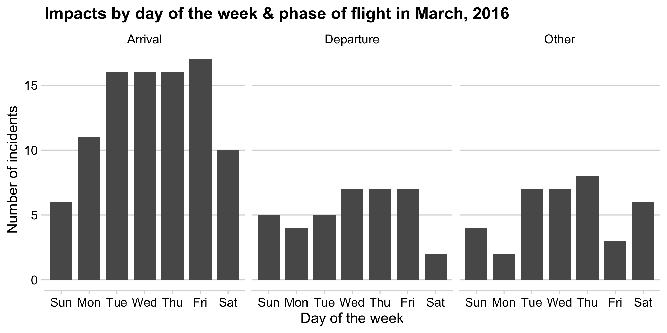
2. Use the lubridate package to create a new variable, weekday_name, from the incident_date variable in the wildlife_impacts data.

3. Use weekday_name and phase_of_flt to make this plot of “arrival” and “departure” impacts from Mar. 2016.

Week 5: Joins & Data Cleaning

1. Merging datasets with joins

2. Are your variables the right type?

3. Are your variables the right name?

4. Re-coding variables

5. Dates

6. Dealing with messy Excel files

Reminders:

• You have 11 days until your Mini Project 1 is due.
• Look at HW 4, due next week
• Quiz 2 next week

When columns are repeated

Example: Winners of Nathan’s hot dog eating contest

Stragies

1. divide & conquer

2. pivot long, separate, pivot wide

Strategy 1: divide & conquer

Steps:

1. Read in the data
2. Clean the names
3. Remove * note at bottom of table

hot_dogs <- read_excel(
  file.path('data', 'hot_dog_winners.xlsx'),
  sheet = 'hot_dog_winners'
) %>%
  clean_names() %>%
  dplyr::filter(!is.na(mens))

glimpse(hot_dogs)

#> Rows: 40
#> Columns: 7
#> $ year         <chr> "1980", "1981", "1982", "1983", "1984", "1985", "1986", "1987", "1988", "1989", "1990", "1991", "1992", "1993", "1994", "1995", "1996", "1997", "1998", "1999", "2000", "2001", "2002", "2003", "2004", "2005", "2006", "2007", "20…
#> $ mens         <chr> "Paul Siederman & Joe Baldini", "Thomas DeBerry", "Steven Abrams", "Luis Llamas", "Birgit Felden", "Oscar Rodriguez", "Mark Heller", "Don Wolfman", "Jay Green", "Jay Green", "Mike DeVito", "Frank Dellarosa", "Frank Dellarosa", …
#> $ dogs_eaten_3 <chr> "9.1", "11", "11", "19.5", "9.5", "11.75", "15.5", "12", "14", "13", "16", "21.5*", "19", "17", "20", "19.5", "22.25*", "24.5*", "19", "20.25", "25.13*", "50*", "50.5*", "44.5", "53.5*", "49", "53.75*", "66*", "59", "68*", "54"…
#> $ country_4    <chr> "United States", "United States", "United States", "Mexico", "Germany", "United States", "United States", "United States", "United States", "United States", "United States", "United States", "United States", "United States", "U…
#> $ womens       <chr> NA, NA, NA, NA, NA, NA, NA, NA, NA, NA, NA, NA, NA, NA, NA, NA, NA, NA, NA, NA, NA, NA, NA, NA, NA, NA, NA, NA, NA, NA, NA, "Sonya Thomas", "Sonya Thomas", "Sonya Thomas", "Miki Sudo", "Miki Sudo", "Miki Sudo", "Miki Sudo", "Mi…
#> $ dogs_eaten_6 <chr> NA, NA, NA, NA, NA, NA, NA, NA, NA, NA, NA, NA, NA, NA, NA, NA, NA, NA, NA, NA, NA, NA, NA, NA, NA, NA, NA, NA, NA, NA, NA, "40*", "45*", "36.75", "34", "38", "38.5", "41", "37", "31"
#> $ country_7    <chr> NA, NA, NA, NA, NA, NA, NA, NA, NA, NA, NA, NA, NA, NA, NA, NA, NA, NA, NA, NA, NA, NA, NA, NA, NA, NA, NA, NA, NA, NA, NA, "United States", "United States", "United States", "United States", "United States", "United States", "…

Strategy 1: divide & conquer

Steps

1. Read in the data
2. Clean the names
3. Remove * note at bottom of table
4. Split data into two competitions with the same variable names
5. Create new variable in each data frame: competition

hot_dogs_m <- hot_dogs %>%
  select(
    year,
    competitor = mens,
    dogs_eaten = dogs_eaten_3,
    country = country_4
  ) %>%
  mutate(competition = 'Mens')

hot_dogs_w <- hot_dogs %>%
  select(
    year,
    competitor = womens,
    dogs_eaten = dogs_eaten_6,
    country = country_7
  ) %>%
  mutate(competition = 'Womens') %>%
  dplyr::filter(!is.na(competitor))

Strategy 1: divide & conquer

Steps

1. Read in the data
2. Clean the names
3. Remove * note at bottom of table
4. Split data into two competitions with the same variable names
5. Create new variable in each data frame: competition
6. Merge data together with bind_rows()
7. Clean up final data frame

hot_dogs <- bind_rows(hot_dogs_m, hot_dogs_w) %>%
  mutate(
    new_record = str_detect(dogs_eaten, "\\*"),
    dogs_eaten = parse_number(dogs_eaten),
    year = as.numeric(year)
  )

glimpse(hot_dogs)

#> Rows: 49
#> Columns: 6
#> $ year        <dbl> 1980, 1981, 1982, 1983, 1984, 1985, 1986, 1987, 1988, 1989, 1990, 1991, 1992, 1993, 1994, 1995, 1996, 1997, 1998, 1999, 2000, 2001, 2002, 2003, 2004, 2005, 2006, 2007, 2008, 2009, 2010, 2011, 2012, 2013, 2014, 2015, 2016, 2017, …
#> $ competitor  <chr> "Paul Siederman & Joe Baldini", "Thomas DeBerry", "Steven Abrams", "Luis Llamas", "Birgit Felden", "Oscar Rodriguez", "Mark Heller", "Don Wolfman", "Jay Green", "Jay Green", "Mike DeVito", "Frank Dellarosa", "Frank Dellarosa", "…
#> $ dogs_eaten  <dbl> 9.10, 11.00, 11.00, 19.50, 9.50, 11.75, 15.50, 12.00, 14.00, 13.00, 16.00, 21.50, 19.00, 17.00, 20.00, 19.50, 22.25, 24.50, 19.00, 20.25, 25.13, 50.00, 50.50, 44.50, 53.50, 49.00, 53.75, 66.00, 59.00, 68.00, 54.00, 62.00, 68.00,…
#> $ country     <chr> "United States", "United States", "United States", "Mexico", "Germany", "United States", "United States", "United States", "United States", "United States", "United States", "United States", "United States", "United States", "Un…
#> $ competition <chr> "Mens", "Mens", "Mens", "Mens", "Mens", "Mens", "Mens", "Mens", "Mens", "Mens", "Mens", "Mens", "Mens", "Mens", "Mens", "Mens", "Mens", "Mens", "Mens", "Mens", "Mens", "Mens", "Mens", "Mens", "Mens", "Mens", "Mens", "Mens", "Men…
#> $ new_record  <lgl> FALSE, FALSE, FALSE, FALSE, FALSE, FALSE, FALSE, FALSE, FALSE, FALSE, FALSE, TRUE, FALSE, FALSE, FALSE, FALSE, TRUE, TRUE, FALSE, FALSE, TRUE, TRUE, TRUE, FALSE, TRUE, FALSE, TRUE, TRUE, FALSE, TRUE, FALSE, FALSE, FALSE, TRUE, F…

head(hot_dogs)

#> # A tibble: 6 × 6
#>    year competitor                   dogs_eaten country       competition new_record
#>   <dbl> <chr>                             <dbl> <chr>         <chr>       <lgl>     
#> 1  1980 Paul Siederman & Joe Baldini        9.1 United States Mens        FALSE     
#> 2  1981 Thomas DeBerry                     11   United States Mens        FALSE     
#> 3  1982 Steven Abrams                      11   United States Mens        FALSE     
#> 4  1983 Luis Llamas                        19.5 Mexico        Mens        FALSE     
#> 5  1984 Birgit Felden                       9.5 Germany       Mens        FALSE     
#> 6  1985 Oscar Rodriguez                    11.8 United States Mens        FALSE

Strategy 2: pivot long, separate, pivot wide

Steps:

1. Read in the data
2. Clean the names
3. Remove * note at bottom of table

hot_dogs <- read_excel(
  file.path('data', 'hot_dog_winners.xlsx'),
  sheet = 'hot_dog_winners'
) %>%
  clean_names() %>%
  dplyr::filter(!is.na(mens))

glimpse(hot_dogs)

#> Rows: 40
#> Columns: 7
#> $ year         <chr> "1980", "1981", "1982", "1983", "1984", "1985", "1986", "1987", "1988", "1989", "1990", "1991", "1992", "1993", "1994", "1995", "1996", "1997", "1998", "1999", "2000", "2001", "2002", "2003", "2004", "2005", "2006", "2007", "20…
#> $ mens         <chr> "Paul Siederman & Joe Baldini", "Thomas DeBerry", "Steven Abrams", "Luis Llamas", "Birgit Felden", "Oscar Rodriguez", "Mark Heller", "Don Wolfman", "Jay Green", "Jay Green", "Mike DeVito", "Frank Dellarosa", "Frank Dellarosa", …
#> $ dogs_eaten_3 <chr> "9.1", "11", "11", "19.5", "9.5", "11.75", "15.5", "12", "14", "13", "16", "21.5*", "19", "17", "20", "19.5", "22.25*", "24.5*", "19", "20.25", "25.13*", "50*", "50.5*", "44.5", "53.5*", "49", "53.75*", "66*", "59", "68*", "54"…
#> $ country_4    <chr> "United States", "United States", "United States", "Mexico", "Germany", "United States", "United States", "United States", "United States", "United States", "United States", "United States", "United States", "United States", "U…
#> $ womens       <chr> NA, NA, NA, NA, NA, NA, NA, NA, NA, NA, NA, NA, NA, NA, NA, NA, NA, NA, NA, NA, NA, NA, NA, NA, NA, NA, NA, NA, NA, NA, NA, "Sonya Thomas", "Sonya Thomas", "Sonya Thomas", "Miki Sudo", "Miki Sudo", "Miki Sudo", "Miki Sudo", "Mi…
#> $ dogs_eaten_6 <chr> NA, NA, NA, NA, NA, NA, NA, NA, NA, NA, NA, NA, NA, NA, NA, NA, NA, NA, NA, NA, NA, NA, NA, NA, NA, NA, NA, NA, NA, NA, NA, "40*", "45*", "36.75", "34", "38", "38.5", "41", "37", "31"
#> $ country_7    <chr> NA, NA, NA, NA, NA, NA, NA, NA, NA, NA, NA, NA, NA, NA, NA, NA, NA, NA, NA, NA, NA, NA, NA, NA, NA, NA, NA, NA, NA, NA, NA, "United States", "United States", "United States", "United States", "United States", "United States", "…

Strategy 2: pivot long, separate, pivot wide

Steps:

1. Read in the data
2. Clean the names
3. Remove * note at bottom of table
4. Rename variables
5. Gather all the “joint” variables

hot_dogs <- hot_dogs %>%
  select(
    year,
    competitor.mens = mens,
    competitor.womens = womens,
    dogs_eaten.mens = dogs_eaten_3,
    dogs_eaten.womens = dogs_eaten_6,
    country.mens = country_4,
    country.womens = country_7
  ) %>%
  pivot_longer(
    names_to = 'variable',
    values_to = 'value',
    competitor.mens:country.womens
  )

head(hot_dogs, 3)

#> # A tibble: 3 × 3
#>   year  variable          value                       
#>   <chr> <chr>             <chr>                       
#> 1 1980  competitor.mens   Paul Siederman & Joe Baldini
#> 2 1980  competitor.womens <NA>                        
#> 3 1980  dogs_eaten.mens   9.1

Strategy 2: pivot long, separate, pivot wide

Steps:

1. Read in the data
2. Clean the names
3. Remove * note at bottom of table
4. Rename variables
5. Gather all the “joint” variables
6. Separate “joint” variables into components

hot_dogs <- hot_dogs %>%
  separate(
    variable,
    into = c('variable', 'competition'),
    sep = '\\.'
  )

head(hot_dogs)

#> # A tibble: 6 × 4
#>   year  variable   competition value                       
#>   <chr> <chr>      <chr>       <chr>                       
#> 1 1980  competitor mens        Paul Siederman & Joe Baldini
#> 2 1980  competitor womens      <NA>                        
#> 3 1980  dogs_eaten mens        9.1                         
#> 4 1980  dogs_eaten womens      <NA>                        
#> 5 1980  country    mens        United States               
#> 6 1980  country    womens      <NA>

Strategy 2: pivot long, separate, pivot wide

Steps:

1. Read in the data
2. Clean the names
3. Remove * note at bottom of table
4. Rename variables
5. Gather all the “joint” variables
6. Separate “joint” variables into components
7. Spread variable and value back to columns
8. Clean up final data frame

hot_dogs <- hot_dogs %>%
  pivot_wider(names_from = variable, values_from = value) %>%
  mutate(
    new_record = str_detect(dogs_eaten, "\\*"),
    dogs_eaten = parse_number(dogs_eaten),
    year = as.numeric(year)
  )

glimpse(hot_dogs)

#> Rows: 80
#> Columns: 6
#> $ year        <dbl> 1980, 1980, 1981, 1981, 1982, 1982, 1983, 1983, 1984, 1984, 1985, 1985, 1986, 1986, 1987, 1987, 1988, 1988, 1989, 1989, 1990, 1990, 1991, 1991, 1992, 1992, 1993, 1993, 1994, 1994, 1995, 1995, 1996, 1996, 1997, 1997, 1998, 1998, …
#> $ competition <chr> "mens", "womens", "mens", "womens", "mens", "womens", "mens", "womens", "mens", "womens", "mens", "womens", "mens", "womens", "mens", "womens", "mens", "womens", "mens", "womens", "mens", "womens", "mens", "womens", "mens", "wom…
#> $ competitor  <chr> "Paul Siederman & Joe Baldini", NA, "Thomas DeBerry", NA, "Steven Abrams", NA, "Luis Llamas", NA, "Birgit Felden", NA, "Oscar Rodriguez", NA, "Mark Heller", NA, "Don Wolfman", NA, "Jay Green", NA, "Jay Green", NA, "Mike DeVito",…
#> $ dogs_eaten  <dbl> 9.10, NA, 11.00, NA, 11.00, NA, 19.50, NA, 9.50, NA, 11.75, NA, 15.50, NA, 12.00, NA, 14.00, NA, 13.00, NA, 16.00, NA, 21.50, NA, 19.00, NA, 17.00, NA, 20.00, NA, 19.50, NA, 22.25, NA, 24.50, NA, 19.00, NA, 20.25, NA, 25.13, NA,…
#> $ country     <chr> "United States", NA, "United States", NA, "United States", NA, "Mexico", NA, "Germany", NA, "United States", NA, "United States", NA, "United States", NA, "United States", NA, "United States", NA, "United States", NA, "United St…
#> $ new_record  <lgl> FALSE, NA, FALSE, NA, FALSE, NA, FALSE, NA, FALSE, NA, FALSE, NA, FALSE, NA, FALSE, NA, FALSE, NA, FALSE, NA, FALSE, NA, TRUE, NA, FALSE, NA, FALSE, NA, FALSE, NA, FALSE, NA, TRUE, NA, TRUE, NA, FALSE, NA, FALSE, NA, TRUE, NA, T…

Divide & conquer

hot_dogs <- read_excel(
  file.path('data', 'hot_dog_winners.xlsx'),
  sheet = 'hot_dog_winners'
) %>%
  clean_names() %>%
  dplyr::filter(!is.na(mens))

# Divide
hot_dogs_m <- hot_dogs %>%
  select(
    year,
    competitor = mens,
    dogs_eaten = dogs_eaten_3,
    country = country_4
  ) %>%
  mutate(competition = 'Mens')
hot_dogs_w <- hot_dogs %>%
  select(
    year,
    competitor = womens,
    dogs_eaten = dogs_eaten_6,
    country = country_7
  ) %>%
  mutate(competition = 'Womens') %>%
  dplyr::filter(!is.na(competitor))

# Merge and finish cleaning
hot_dogs <- bind_rows(hot_dogs_m, hot_dogs_w) %>%
  mutate(
    new_record = str_detect(dogs_eaten, "\\*"),
    dogs_eaten = parse_number(dogs_eaten),
    year = as.numeric(year)
  )

Pivot long, separate, pivot wide

hot_dogs <- read_excel(
  file.path('data', 'hot_dog_winners.xlsx'),
  sheet = 'hot_dog_winners'
) %>%
  clean_names() %>%
  dplyr::filter(!is.na(mens)) %>%

  # Rename variables
  select(
    year,
    competitor.mens = mens,
    competitor.womens = womens,
    dogs_eaten.mens = dogs_eaten_3,
    dogs_eaten.womens = dogs_eaten_6,
    country.mens = country_4,
    country.womens = country_7
  ) %>%
  # Gather "joint" variables
  pivot_longer(
    names_to = 'variable',
    values_to = 'value',
    competitor.mens:country.womens
  ) %>%
  # Separate "joint" variables
  separate(variable, into = c('variable', 'competition'), sep = '\\.') %>%
  # Spread "joint" variables
  pivot_wider(names_from = variable, values_from = value) %>%
  # Finish cleaning
  mutate(
    new_record = str_detect(dogs_eaten, "\\*"),
    dogs_eaten = parse_number(dogs_eaten),
    year = as.numeric(year)
  )

Strategies for dealing with sub-headers

Example:

OICA passenger car sales data

Strategies for dealing with sub-headers

Steps:

1. Read in the data, skipping first 5 rows
2. Clean the names

pc_sales <- read_excel(
  file.path('data', 'pc_sales_2018.xlsx'),
  sheet = 'pc_sales',
  skip = 5
) %>%
  clean_names() %>%
  rename(country = regions_countries)

glimpse(pc_sales)

#> Rows: 160
#> Columns: 18
#> $ country <chr> NA, "EUROPE", "EU 28 countries + EFTA", "EU 15 countries + EFTA", "AUSTRIA", "BELGIUM", "DENMARK", "FINLAND", "FRANCE", "GERMANY", "GREECE", "ICELAND", "IRELAND", "ITALY", "LUXEMBOURG", "NETHERLANDS", "NORWAY", "PORTUGAL", "SPAIN", …
#> $ x2      <lgl> NA, NA, NA, NA, NA, NA, NA, NA, NA, NA, NA, NA, NA, NA, NA, NA, NA, NA, NA, NA, NA, NA, NA, NA, NA, NA, NA, NA, NA, NA, NA, NA, NA, NA, NA, NA, NA, NA, NA, NA, NA, NA, NA, NA, NA, NA, NA, NA, NA, NA, NA, NA, NA, NA, NA, NA, NA, NA, …
#> $ x3      <lgl> NA, NA, NA, NA, NA, NA, NA, NA, NA, NA, NA, NA, NA, NA, NA, NA, NA, NA, NA, NA, NA, NA, NA, NA, NA, NA, NA, NA, NA, NA, NA, NA, NA, NA, NA, NA, NA, NA, NA, NA, NA, NA, NA, NA, NA, NA, NA, NA, NA, NA, NA, NA, NA, NA, NA, NA, NA, NA, …
#> $ x4      <lgl> NA, NA, NA, NA, NA, NA, NA, NA, NA, NA, NA, NA, NA, NA, NA, NA, NA, NA, NA, NA, NA, NA, NA, NA, NA, NA, NA, NA, NA, NA, NA, NA, NA, NA, NA, NA, NA, NA, NA, NA, NA, NA, NA, NA, NA, NA, NA, NA, NA, NA, NA, NA, NA, NA, NA, NA, NA, NA, …
#> $ x2005   <dbl> NA, 17906455, 15622035, 14565695, 307915, 480088, 148819, 148161, 2118042, 3319259, 269728, 18060, 171742, 2244108, 48517, 465196, 109907, 206488, 1528877, 274301, 266770, 2439717, 1056340, 25956, 70541, 17687, 151699, 19640, 198982…
#> $ x2006   <dbl> NA, 18685556, 15961138, 14820182, 308594, 526141, 156936, 145700, 2045745, 3467961, 267669, 17129, 178484, 2335462, 50837, 483999, 109164, 194702, 1634608, 282766, 269421, 2344864, 1140956, 36455, 78775, 18639, 156686, 25363, 187676…
#> $ x2007   <dbl> NA, 19618588, 16147274, 14842186, 298182, 524795, 162686, 125608, 2109672, 3148163, 279745, 15942, 186325, 2494115, 51332, 504300, 129195, 201816, 1614835, 306794, 284674, 2404007, 1305088, 43521, 82664, 22878, 174456, 30912, 171661…
#> $ x2008   <dbl> NA, 18821599, 14911880, 13602038, 293697, 535947, 150199, 139669, 2091369, 3090040, 267295, 9033, 151607, 2161359, 52359, 499980, 110617, 213389, 1161176, 253982, 288525, 2131795, 1309842, 45143, 88265, 22241, 182554, 24579, 153278,…
#> $ x2009   <dbl> NA, 16608761, 14533115, 13668808, 319403, 476194, 112454, 90574, 2302398, 3807175, 219730, 2113, 57453, 2159465, 47265, 387699, 98675, 161013, 952772, 213408, 266018, 1994999, 864307, 22869, 44918, 14981, 167708, 9946, 60189, 7515, …
#> $ x2010   <dbl> NA, 16499863, 13830694, 12984549, 328563, 547340, 153858, 111968, 2251669, 2916259, 141501, 3106, 88446, 1961580, 49726, 482531, 127754, 223464, 982015, 289684, 294239, 2030846, 846145, 16257, 38587, 14088, 169580, 10295, 43476, 797…
#> $ x2011   <dbl> NA, 17167600, 13642659, 12815435, 356145, 572211, 170036, 126123, 2204229, 3173634, 97680, 5038, 89911, 1749740, 49881, 555812, 138345, 153404, 808051, 304984, 318958, 1941253, 827224, 19250, 41561, 13480, 173595, 17070, 45094, 1323…
#> $ x2012   <dbl> NA, 16191269, 12567903, 11773281, 336010, 486737, 170763, 111251, 1898760, 3082504, 58482, 7902, 79498, 1403010, 50398, 502454, 137967, 95309, 699589, 279899, 328139, 2044609, 794622, 19419, 31360, 10123, 174009, 19424, 53059, 10665…
#> $ x2013   <dbl> NA, 15942273, 12344415, 11555153, 319035, 486065, 182086, 103455, 1790456, 2952431, 58694, 7274, 74367, 1304648, 46624, 417036, 142151, 105921, 722689, 269599, 307885, 2264737, 789262, 19352, 27802, 7102, 164736, 19694, 56139, 10636…
#> $ x2014   <dbl> NA, 16154279, 13061461, 12148648, 303318, 482939, 189055, 106237, 1795885, 3036773, 71218, 9537, 96284, 1360578, 49793, 387553, 144202, 142826, 890125, 303948, 301942, 2476435, 912813, 20359, 33962, 8276, 192314, 20969, 67476, 12452…
#> $ x2015   <dbl> NA, 16410563, 14287881, 13261258, 308555, 501066, 207717, 108819, 1917226, 3206042, 75805, 14004, 124804, 1575737, 46473, 449350, 150686, 178503, 1094077, 345108, 323783, 2633503, 1026623, 23500, 35715, 10344, 230857, 20347, 77171, …
#> $ x2016   <dbl> NA, 17291819, 15160239, 13971468, 329604, 539519, 222924, 118991, 2015177, 3351607, 78873, 18442, 146600, 1824968, 50561, 382825, 154603, 207345, 1147007, 372318, 317318, 2692786, 1188771, 26370, 44106, 12643, 259693, 22429, 96552, …
#> $ x2017   <dbl> NA, 17974281, 15631283, 14320223, 353320, 546558, 221821, 120480, 2110748, 3441262, 88083, 21324, 131332, 1970497, 52775, 414306, 158650, 222129, 1234932, 379393, 311996, 2540617, 1311060, 33265, 50769, 13127, 271595, 25618, 116265,…
#> $ x2018   <dbl> NA, 17912336, 15626509, 14210016, 341068, 549632, 218566, 120480, 2173481, 3435778, 103431, 17976, 125557, 1910025, 52786, 443531, 147929, 228327, 1321438, 353729, 299135, 2367147, 1416493, 37506, 60041, 13135, 261437, 26297, 136601…

Strategies for dealing with sub-headers

Steps:

1. Read in the data, skipping first 5 rows
2. Clean the names
3. Drop bad columns
4. Filter out bad rows

Use datapasta to get rows to drop

drop <- c(
  'EUROPE',
  'EU 28 countries + EFTA',
  'EU 15 countries + EFTA',
  'EUROPE NEW MEMBERS',
  'RUSSIA, TURKEY & OTHER EUROPE',
  'AMERICA',
  'NAFTA',
  'CENTRAL & SOUTH AMERICA',
  'ASIA/OCEANIA/MIDDLE EAST',
  'AFRICA',
  'ALL COUNTRIES'
)

pc_sales <- pc_sales %>%
  select(-c(x2:x4)) %>% # Drop bad columns
  filter(
    !country %in% drop, # Drop bad rows
    !is.na(country)
  )

head(pc_sales)

#> # A tibble: 6 × 15
#>   country   x2005   x2006   x2007   x2008   x2009   x2010   x2011   x2012   x2013   x2014   x2015   x2016   x2017   x2018
#>   <chr>     <dbl>   <dbl>   <dbl>   <dbl>   <dbl>   <dbl>   <dbl>   <dbl>   <dbl>   <dbl>   <dbl>   <dbl>   <dbl>   <dbl>
#> 1 AUSTRIA  307915  308594  298182  293697  319403  328563  356145  336010  319035  303318  308555  329604  353320  341068
#> 2 BELGIUM  480088  526141  524795  535947  476194  547340  572211  486737  486065  482939  501066  539519  546558  549632
#> 3 DENMARK  148819  156936  162686  150199  112454  153858  170036  170763  182086  189055  207717  222924  221821  218566
#> 4 FINLAND  148161  145700  125608  139669   90574  111968  126123  111251  103455  106237  108819  118991  120480  120480
#> 5 FRANCE  2118042 2045745 2109672 2091369 2302398 2251669 2204229 1898760 1790456 1795885 1917226 2015177 2110748 2173481
#> 6 GERMANY 3319259 3467961 3148163 3090040 3807175 2916259 3173634 3082504 2952431 3036773 3206042 3351607 3441262 3435778

Strategies for dealing with sub-headers

Steps:

1. Read in the data, skipping first 5 rows
2. Clean the names
3. Drop bad columns
4. Filter out bad rows
5. Gather the year variables

pc_sales <- pc_sales %>%
  pivot_longer(
    names_to = 'year',
    values_to = 'num_cars',
    cols = x2005:x2018
  )

head(pc_sales)

#> # A tibble: 6 × 3
#>   country year  num_cars
#>   <chr>   <chr>    <dbl>
#> 1 AUSTRIA x2005   307915
#> 2 AUSTRIA x2006   308594
#> 3 AUSTRIA x2007   298182
#> 4 AUSTRIA x2008   293697
#> 5 AUSTRIA x2009   319403
#> 6 AUSTRIA x2010   328563

Strategies for dealing with sub-headers

Steps:

1. Read in the data, skipping first 5 rows
2. Clean the names
3. Drop bad columns
4. Filter out bad rows
5. Gather the year variables
6. Separate the “x” from the year

pc_sales <- pc_sales %>%
  separate(
    year,
    into = c('drop', 'year'),
    sep = 'x',
    convert = TRUE
  )

head(pc_sales)

#> # A tibble: 6 × 4
#>   country drop   year num_cars
#>   <chr>   <lgl> <int>    <dbl>
#> 1 AUSTRIA NA     2005   307915
#> 2 AUSTRIA NA     2006   308594
#> 3 AUSTRIA NA     2007   298182
#> 4 AUSTRIA NA     2008   293697
#> 5 AUSTRIA NA     2009   319403
#> 6 AUSTRIA NA     2010   328563

Strategies for dealing with sub-headers

Steps:

1. Read in the data, skipping first 5 rows
2. Clean the names
3. Drop bad columns
4. Filter out bad rows
5. Gather the year variables
6. Separate the “x” from the year
7. Remove the drop column
8. Finish cleaning

pc_sales <- pc_sales %>%
  select(-drop) %>%
  mutate(country = str_to_title(country))

head(pc_sales)

#> # A tibble: 6 × 3
#>   country  year num_cars
#>   <chr>   <int>    <dbl>
#> 1 Austria  2005   307915
#> 2 Austria  2006   308594
#> 3 Austria  2007   298182
#> 4 Austria  2008   293697
#> 5 Austria  2009   319403
#> 6 Austria  2010   328563

What if I wanted to keep the continents?

Strategy: Join a new data frame linking country -> continent

Strategy 1: Find another source

Strategy 2: Hand-make it

pc_regions <- read_csv(file.path(
  "data",
  "pc_regions.csv"
))

head(pc_regions)

#> # A tibble: 6 × 3
#>   country region subregion             
#>   <chr>   <chr>  <chr>                 
#> 1 AUSTRIA EUROPE EU 15 countries + EFTA
#> 2 BELGIUM EUROPE EU 15 countries + EFTA
#> 3 DENMARK EUROPE EU 15 countries + EFTA
#> 4 FINLAND EUROPE EU 15 countries + EFTA
#> 5 FRANCE  EUROPE EU 15 countries + EFTA
#> 6 GERMANY EUROPE EU 15 countries + EFTA

pc_sales <- pc_sales %>%
  left_join(pc_regions)

head(pc_sales)

#> # A tibble: 6 × 5
#>   country  year num_cars region subregion             
#>   <chr>   <int>    <dbl> <chr>  <chr>                 
#> 1 AUSTRIA  2005   307915 EUROPE EU 15 countries + EFTA
#> 2 AUSTRIA  2006   308594 EUROPE EU 15 countries + EFTA
#> 3 AUSTRIA  2007   298182 EUROPE EU 15 countries + EFTA
#> 4 AUSTRIA  2008   293697 EUROPE EU 15 countries + EFTA
#> 5 AUSTRIA  2009   319403 EUROPE EU 15 countries + EFTA
#> 6 AUSTRIA  2010   328563 EUROPE EU 15 countries + EFTA

drop <- c(
  'EUROPE',
  'EU 28 countries + EFTA',
  'EU 15 countries + EFTA',
  'EUROPE NEW MEMBERS',
  'RUSSIA, TURKEY & OTHER EUROPE',
  'AMERICA',
  'NAFTA',
  'CENTRAL & SOUTH AMERICA',
  'ASIA/OCEANIA/MIDDLE EAST',
  'AFRICA',
  'ALL COUNTRIES'
)

pc_regions <- read_csv(file.path("data", "pc_regions.csv"))

pc_sales <- read_excel(
  file.path('data', 'pc_sales_2018.xlsx'),
  sheet = 'pc_sales',
  skip = 5
) %>%
  clean_names() %>%
  rename(country = regions_countries) %>%
  select(-c(x2:x4)) %>% # Drop bad columns
  filter(
    !country %in% drop, # Drop bad rows
    !is.na(country)
  ) %>%
  pivot_longer(
    names_to = 'year',
    values_to = 'num_cars',
    cols = x2005:x2018
  ) %>%
  separate(year, into = c('drop', 'year'), sep = 'x', convert = TRUE) %>%
  select(-drop) %>%
  left_join(pc_regions) %>%
  mutate(
    country = str_to_title(country),
    region = str_to_title(region),
    subregion = str_to_title(subregion)
  )

head(pc_sales)

#> # A tibble: 6 × 5
#>   country  year num_cars region subregion             
#>   <chr>   <int>    <dbl> <chr>  <chr>                 
#> 1 Austria  2005   307915 Europe Eu 15 Countries + Efta
#> 2 Austria  2006   308594 Europe Eu 15 Countries + Efta
#> 3 Austria  2007   298182 Europe Eu 15 Countries + Efta
#> 4 Austria  2008   293697 Europe Eu 15 Countries + Efta
#> 5 Austria  2009   319403 Europe Eu 15 Countries + Efta
#> 6 Austria  2010   328563 Europe Eu 15 Countries + Efta