10:00
Exploring Data
EMSE 4572/6572: Exploratory Data Analysis
John Paul Helveston
September 30, 2026
Quiz 2
Write your name on the quiz!
Rules:
- Work alone; no outside help of any kind is allowed.
- No calculators, no notes, no books, no computers, no phones.

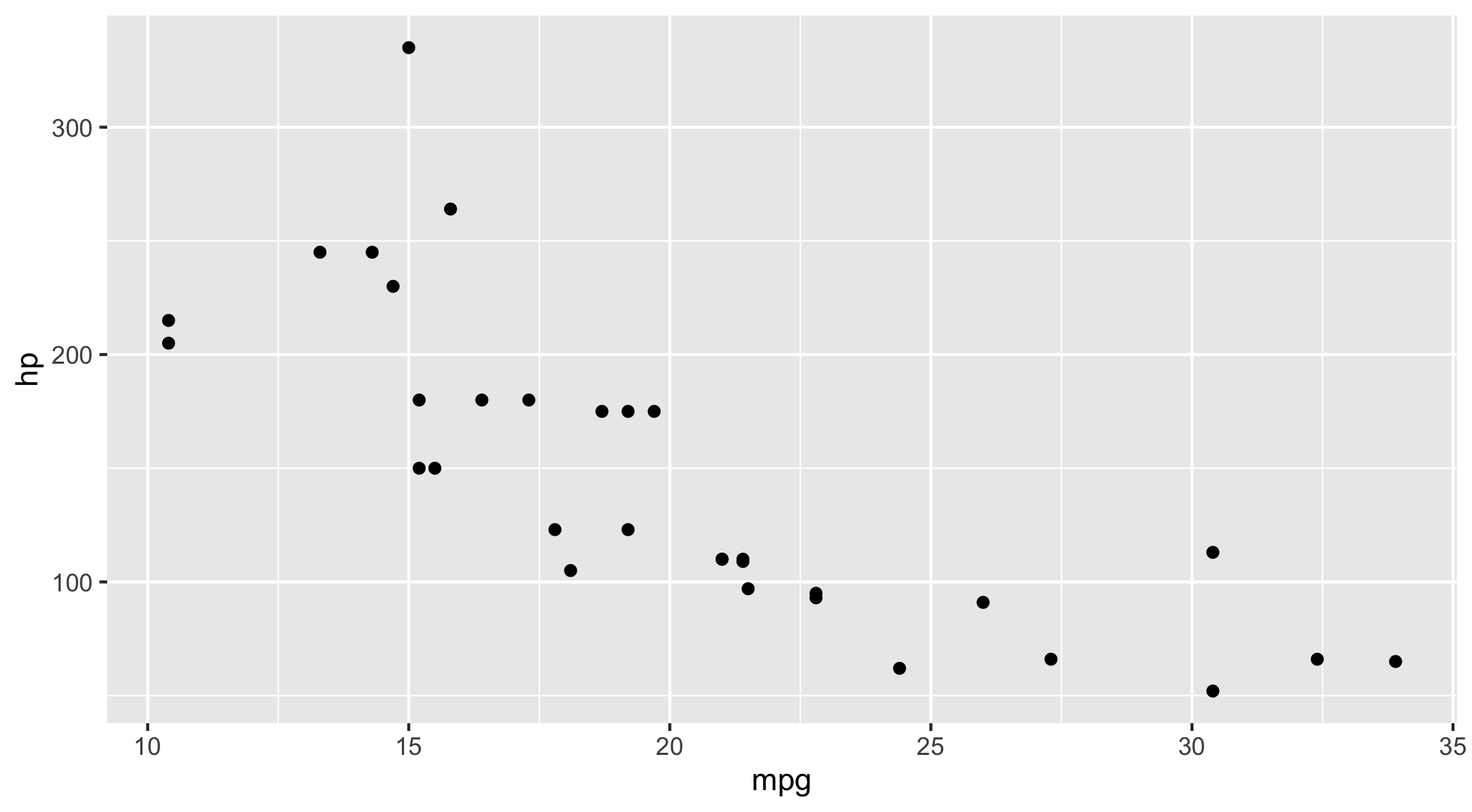
Default theme
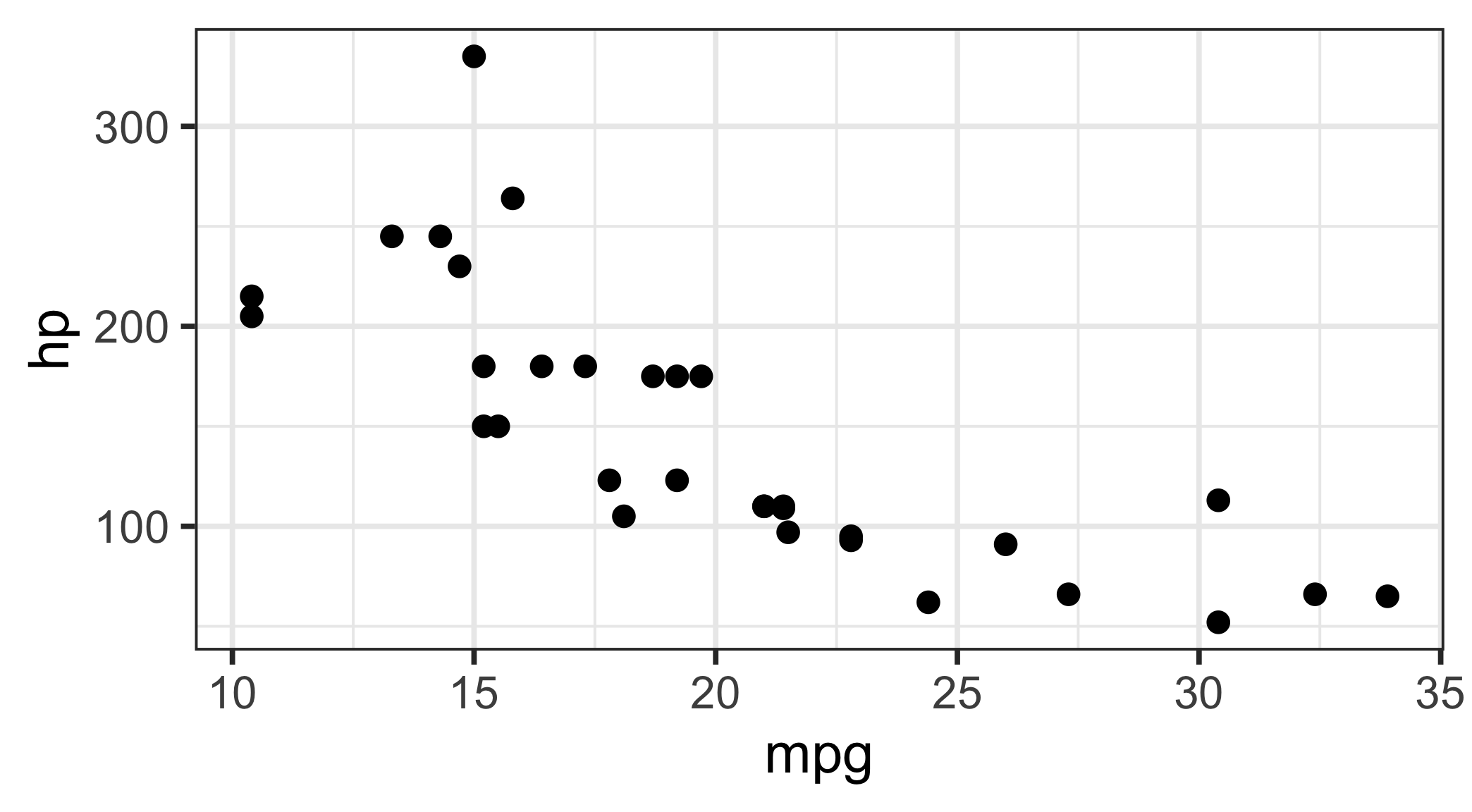
theme_bw(base_size = 20)
Exploratory Analysis
RQ: Do people bike more when the weather is nice?
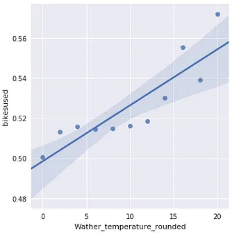
Confirmatory Analysis
Let’s build a model to predict bike usage based on weather.
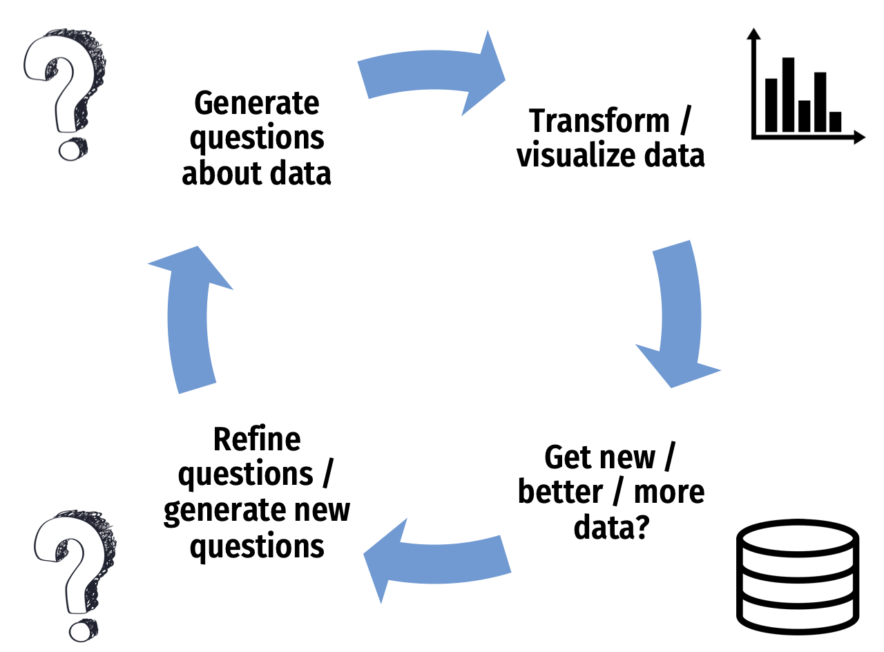
Don’t be Icarus

EDA is an iterative process to help you
understand your data and ask better questions
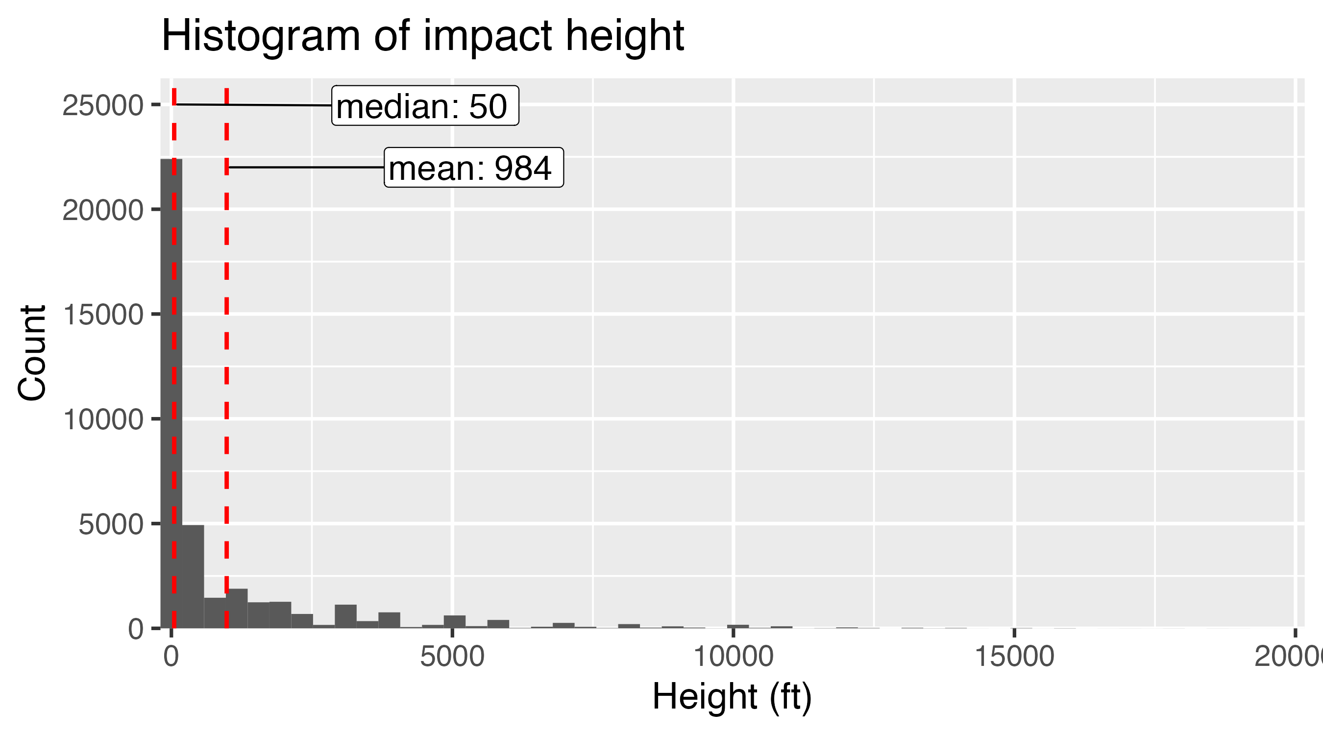
Mean isn’t always the “best” choice
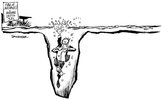
Beware the “flaw of averages”
What happened to the statistician that crossed a river with an average depth of 3 feet?
…he drowned
Example: Days to ship
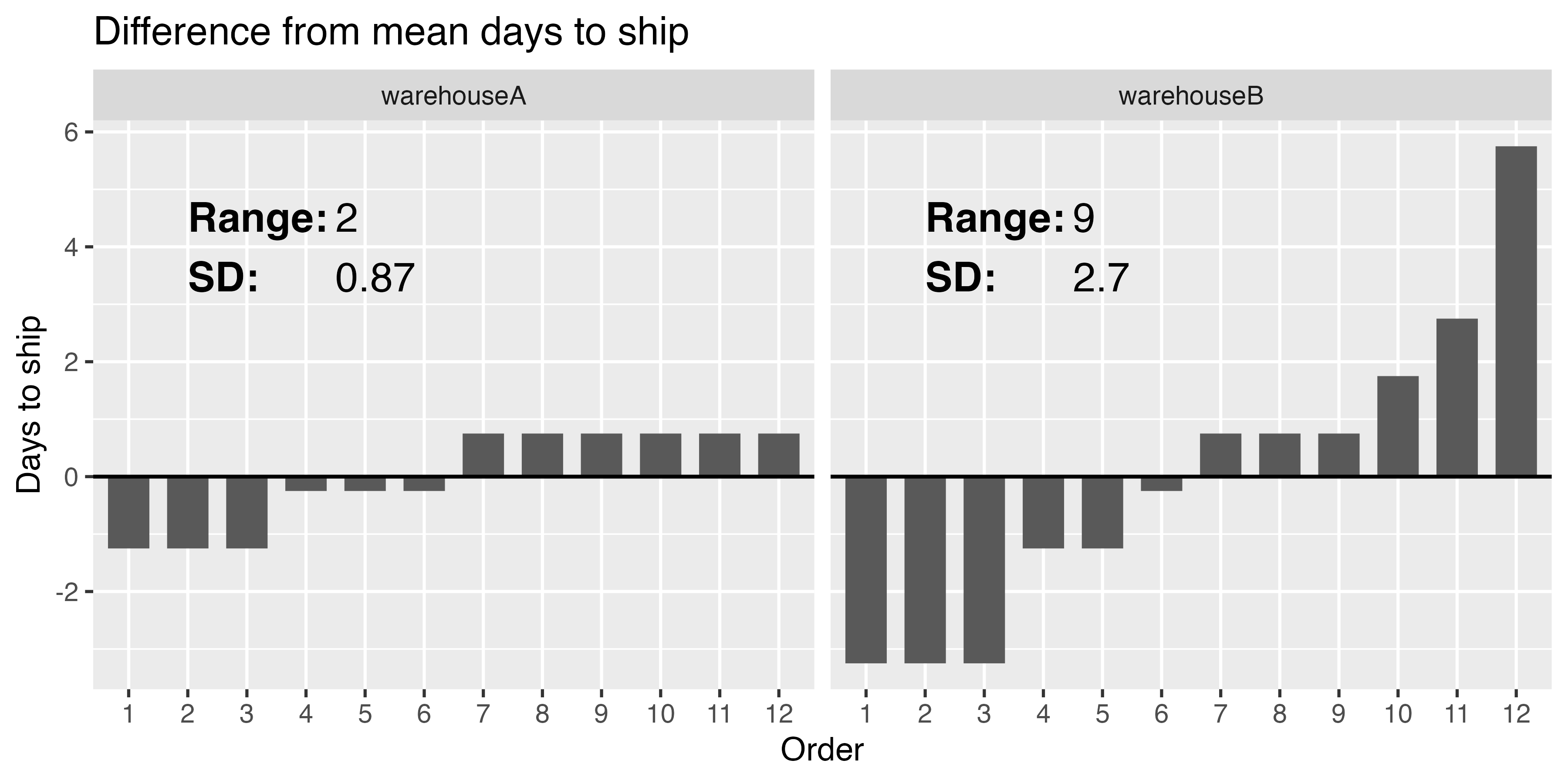
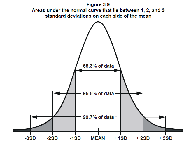
Interpreting the standard deviation
\(s = \sqrt{\frac{\sum_{i=1}^{N}(x_i - \bar{x})^2}{N - 1}}\)
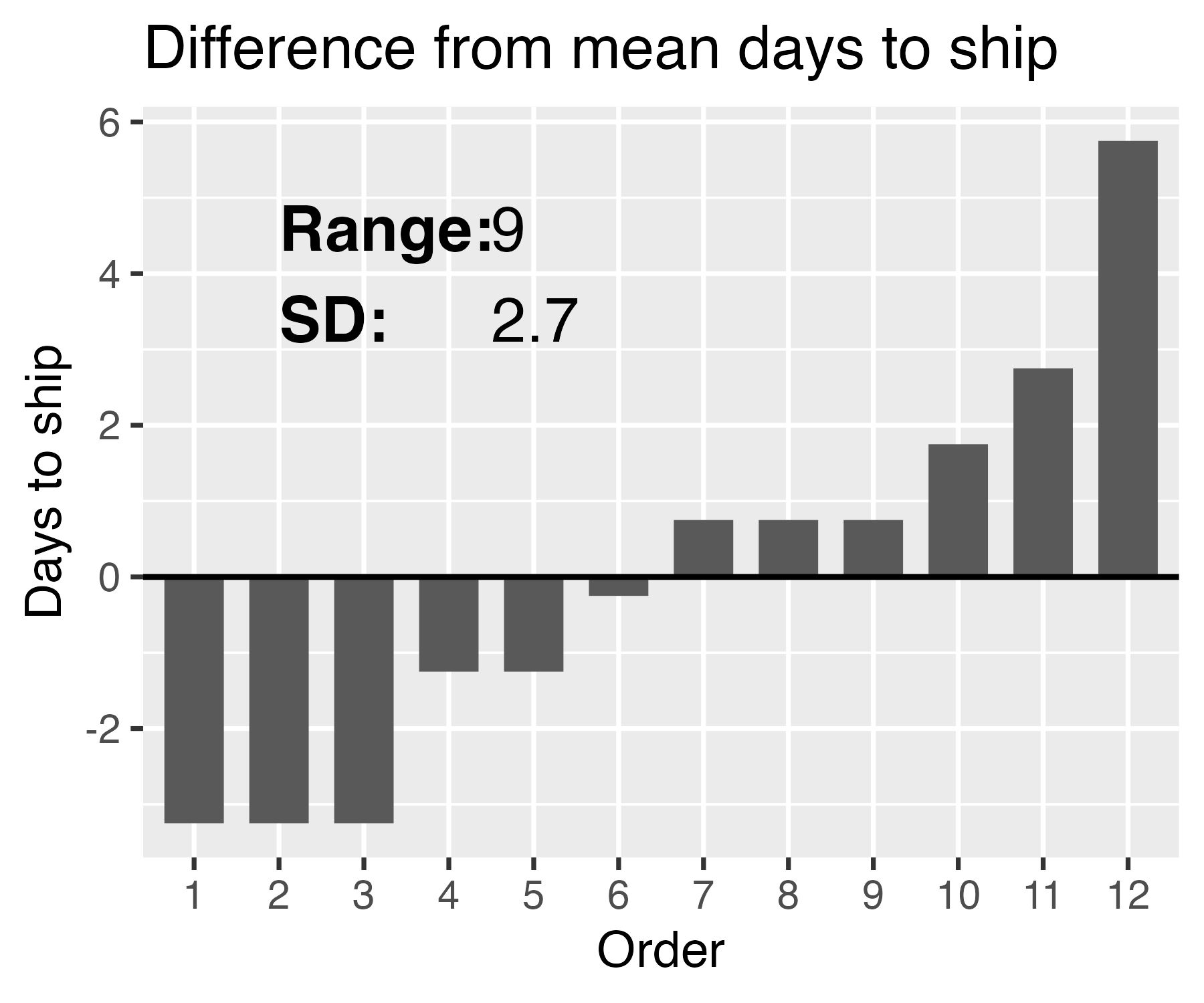
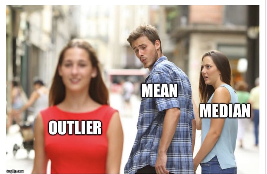
Outliers
“Visualizing data helps us think”
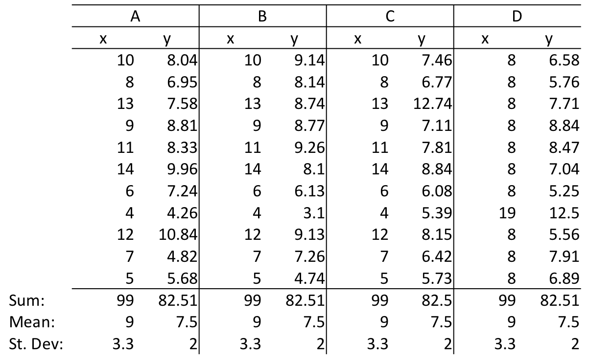
Anscombe’s Quartet
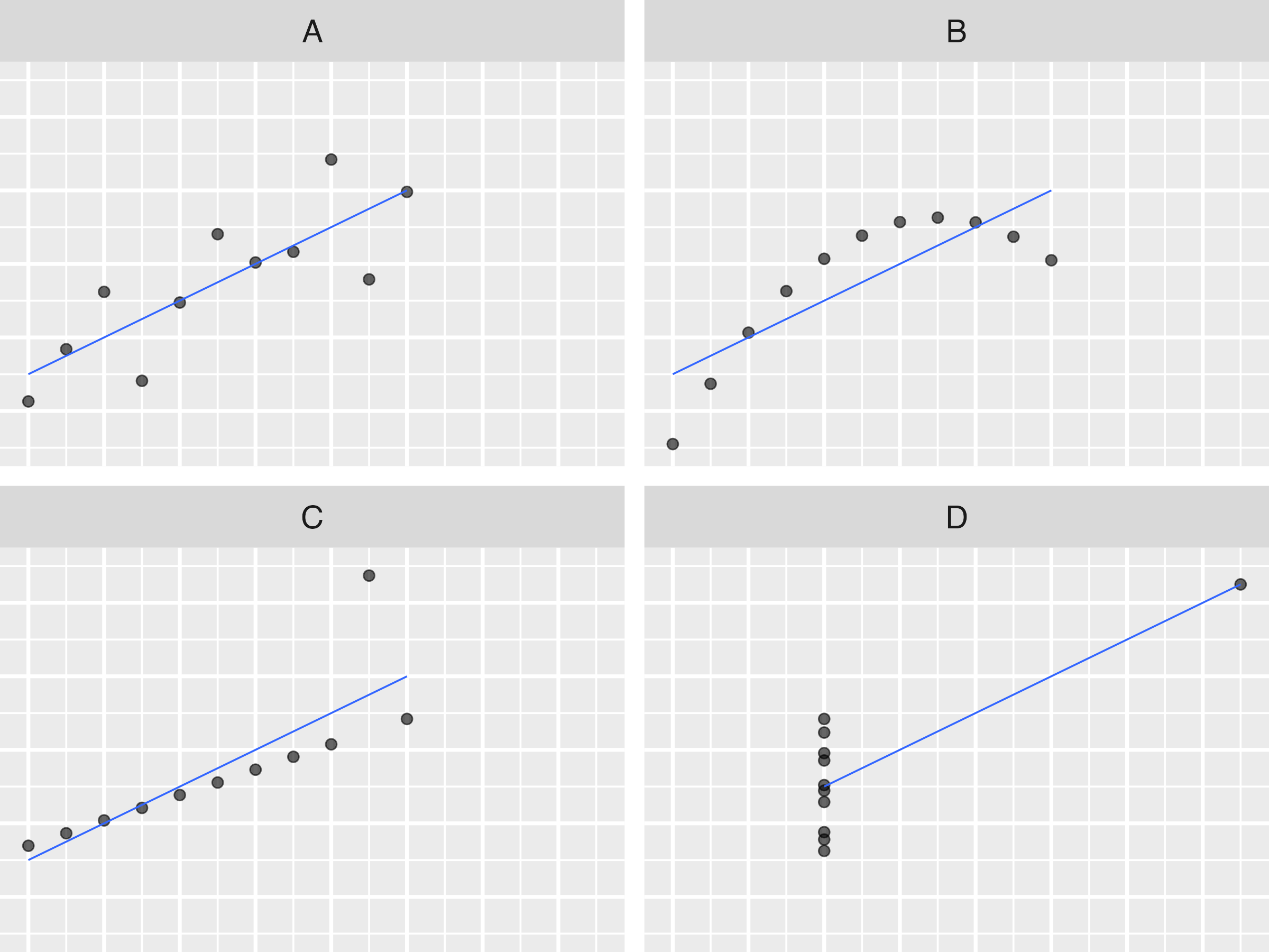
Anscombe’s Quartet
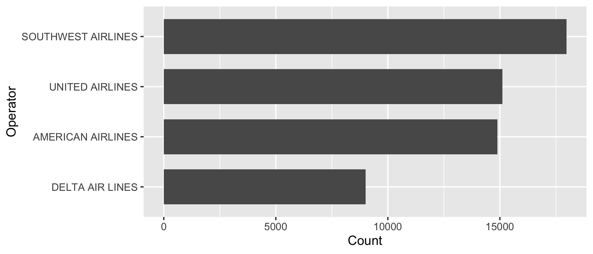
Summarizing Nominal data
Summarize with counts / percentages
Summarizing Ordinal data
Summarize: Counts / percentages
#> # A tibble: 12 × 3
#>    incident_month     n      p
#>             <dbl> <int>  <dbl>
#>  1              9  7980 0.140
#>  2             10  7754 0.136
#>  3              8  7104 0.125
#>  4              5  6161 0.108
#>  5              7  6133 0.108
#>  6              6  4541 0.0797
#>  7              4  4490 0.0788
#>  8             11  4191 0.0736
#>  9              3  2678 0.0470
#> 10             12  2303 0.0404
#> 11              1  1951 0.0342
#> 12              2  1692 0.0297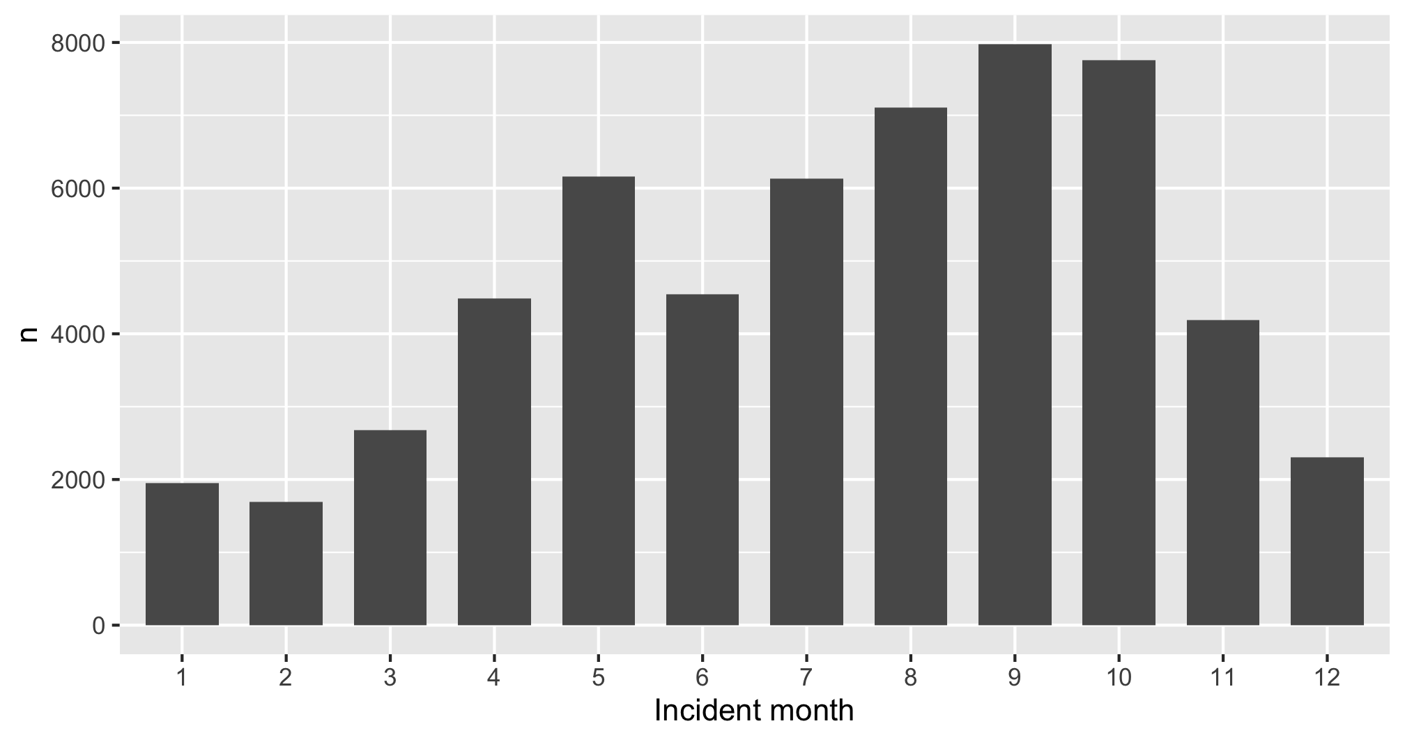
Summarizing continuous variables
Histograms:
- Skewness
- Number of modes
Boxplots:
- Outliers
- Comparing variables
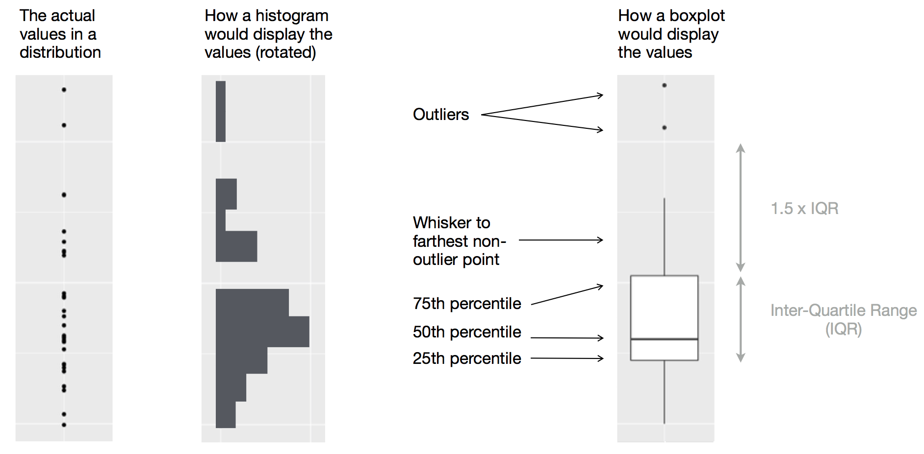
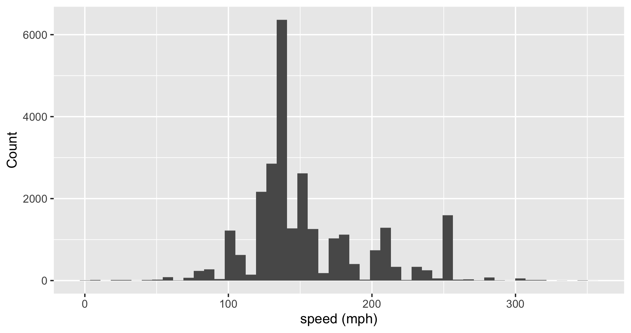
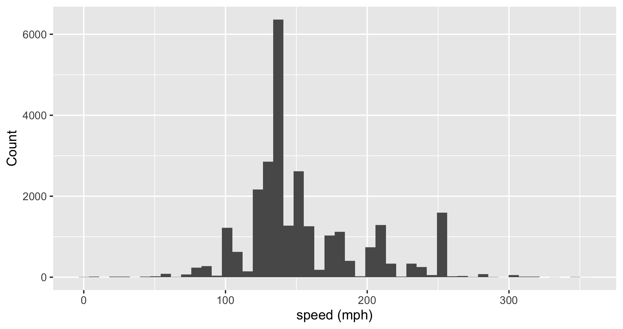
Histogram: Identify Skewness & # of Modes
Summarise:
Mean, median, sd, range, & IQR:
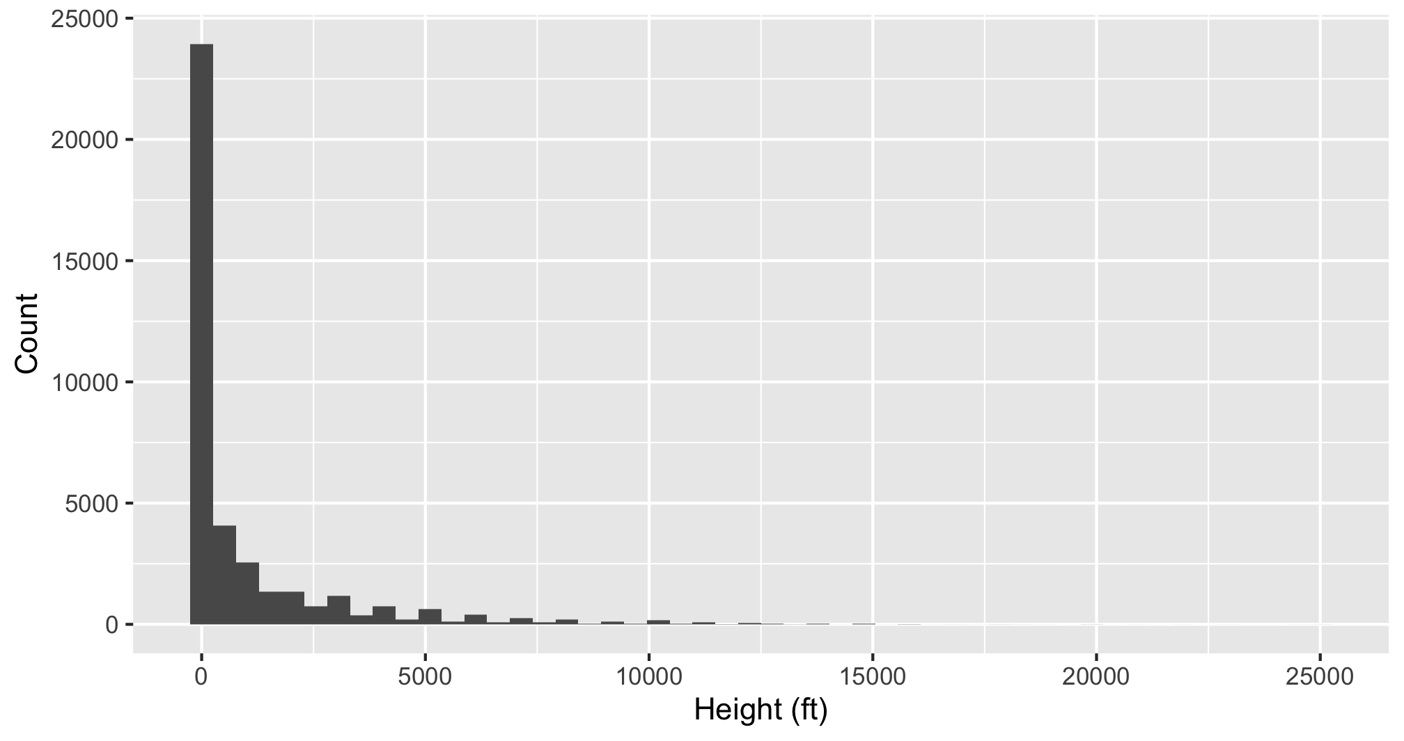
Histogram: Identify Skewness & # of Modes
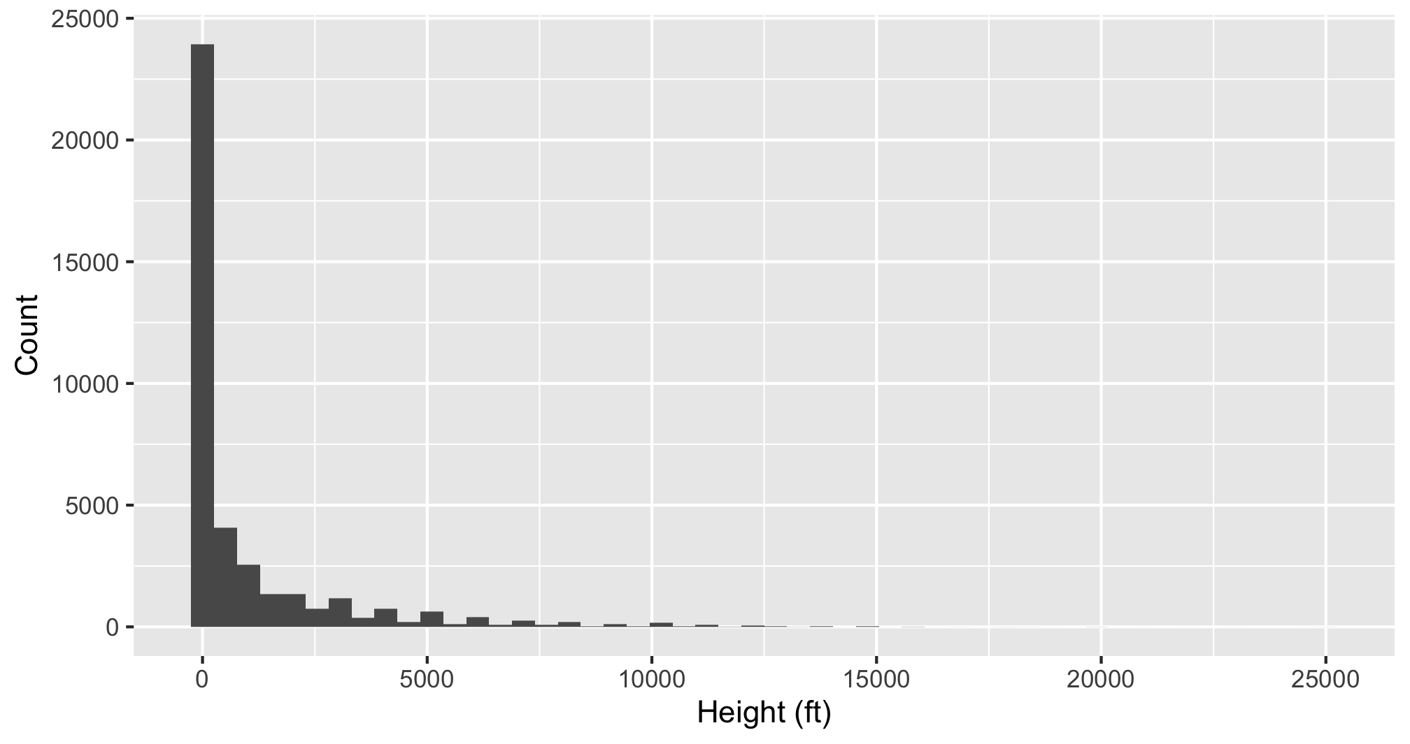
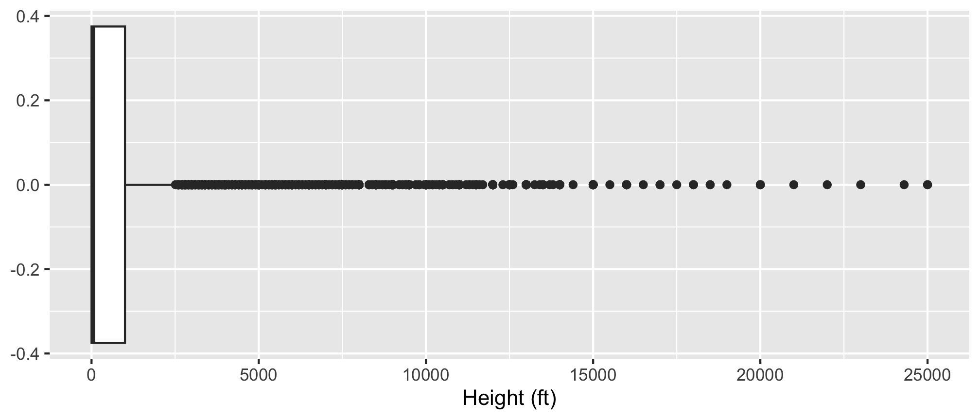
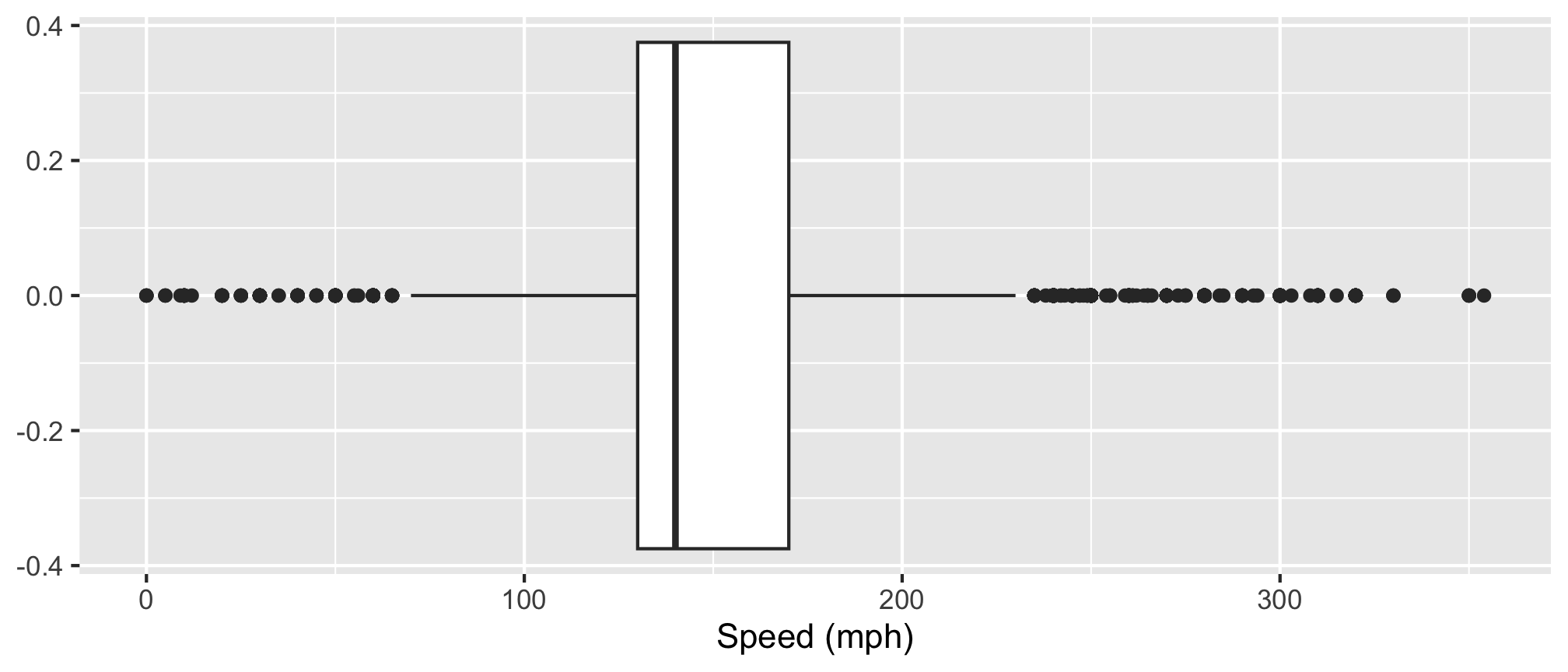
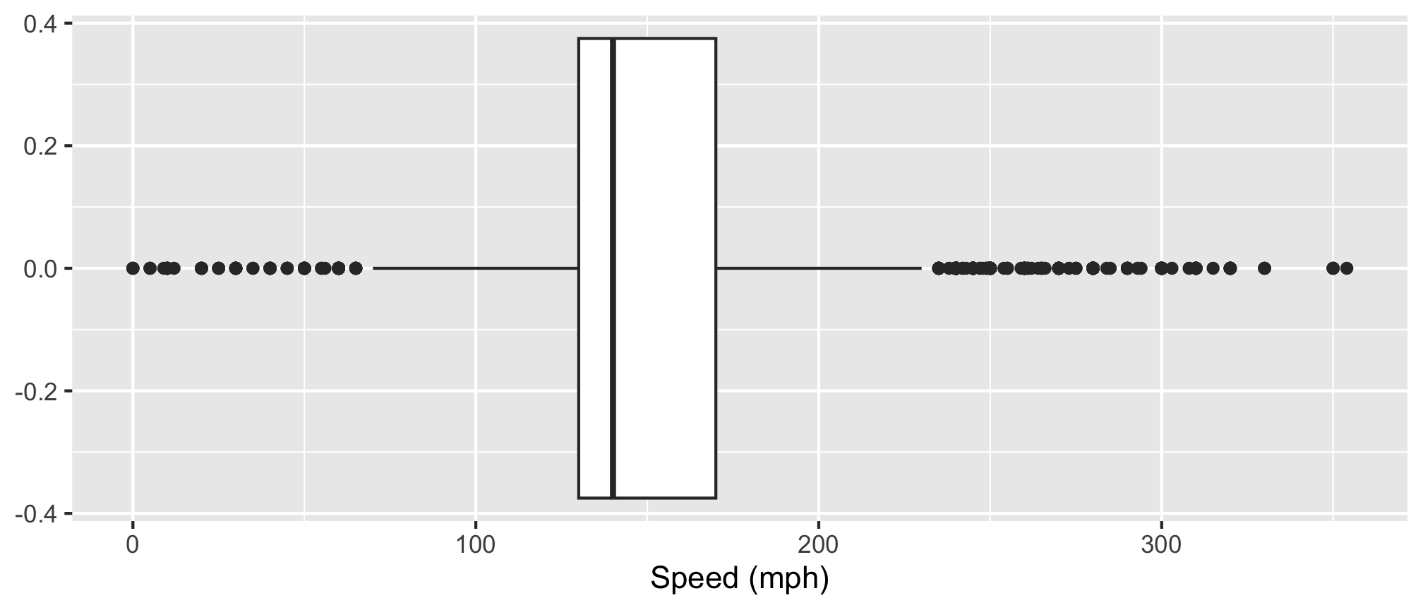
Boxplot: Identify outliers
Histogram
- Skewness
- Modes
Boxplot
- Outliers
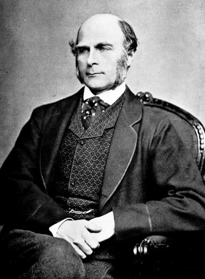
Correlation: a rather racist origin in eugenics (“well born”)
Sir Francis Galton (1822 - 1911)
- Charles Darwin’s cousin.
- “Father” of eugenics.
- Interested in heredity.
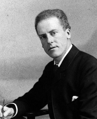
Karl Pearson (1857 - 1936)
- Galton’s (hero-worshiping) protégé.
- Defined correlation equation.
- “Father” of mathematical statistics.
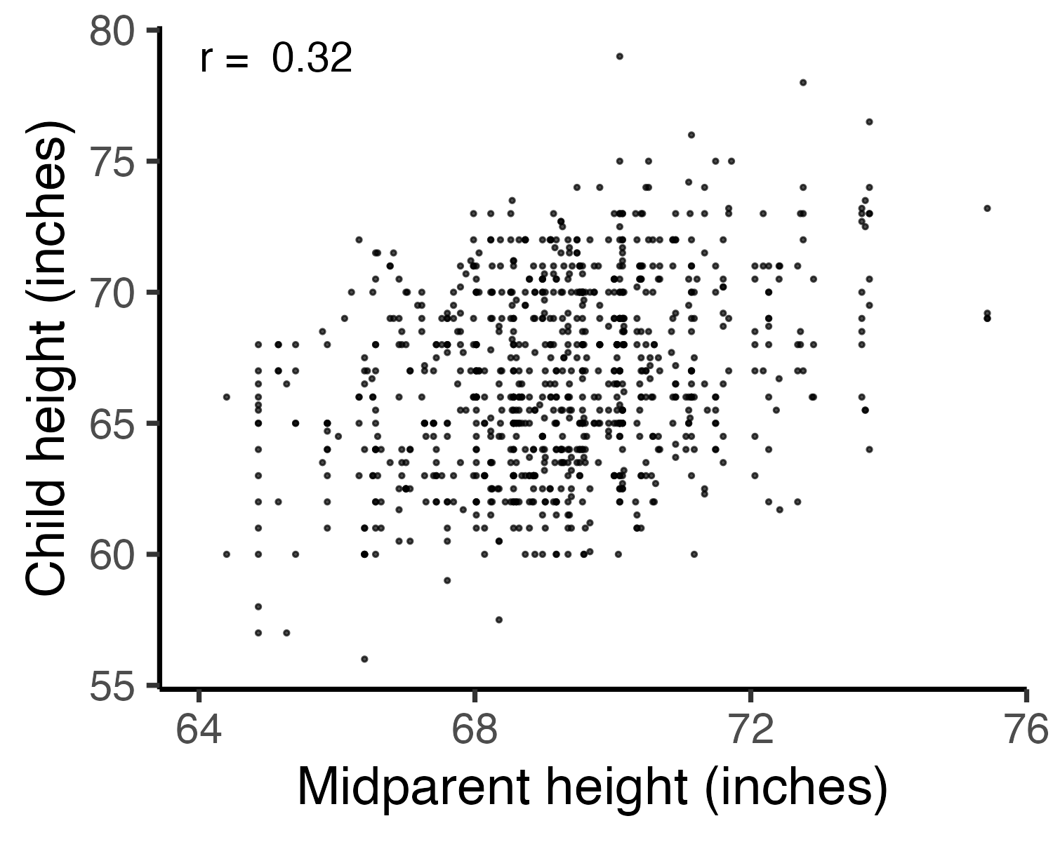
Galton’s family data
Galton, F. (1886). “Regression towards mediocrity in hereditary stature”. The Journal of the Anthropological Institute of Great Britain and Ireland 15: 246-263.
Galton’s question: Does marriage selection indicate a relationship between the heights of husbands and wives?
(He called this “assortative mating”)
“midparent height” is just a scaled mean:
How do you measure correlation?
\(r = \frac{\text{Cov}(x, y)}{\text{sd}(x) * \text{sd}(y)}\)
Assumptions:
- Variables must be interval or ratio
- Linear relationship
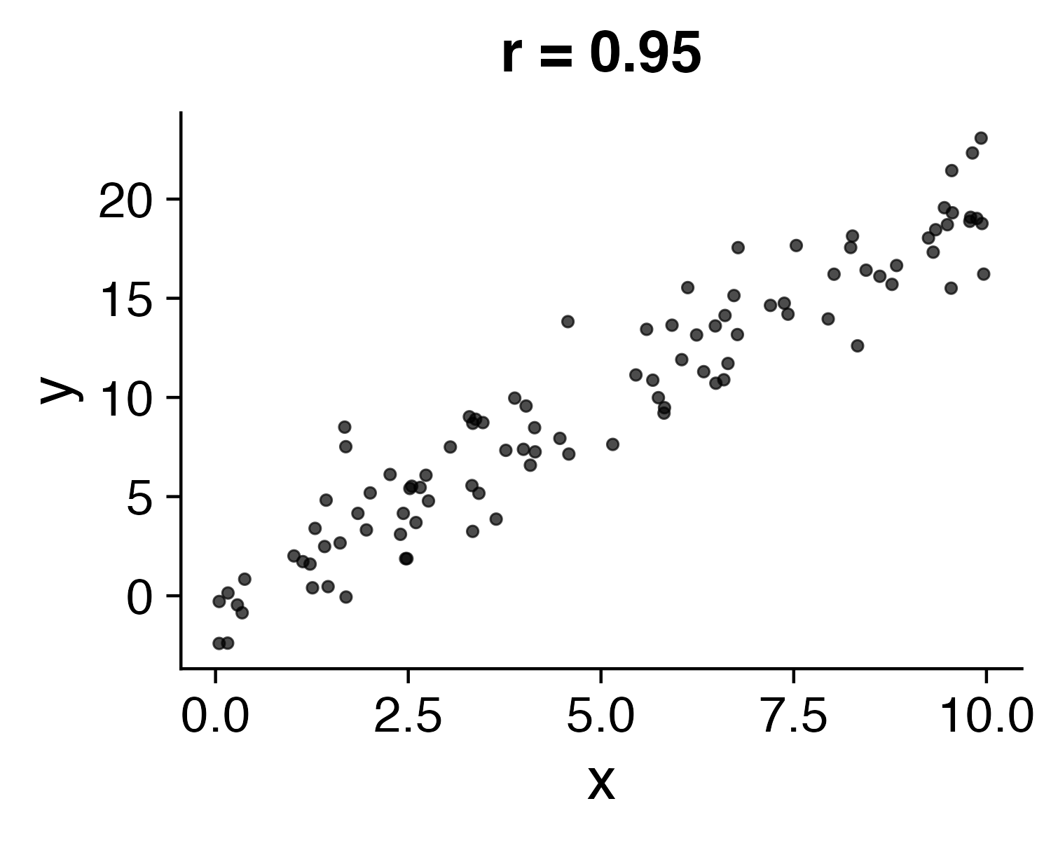
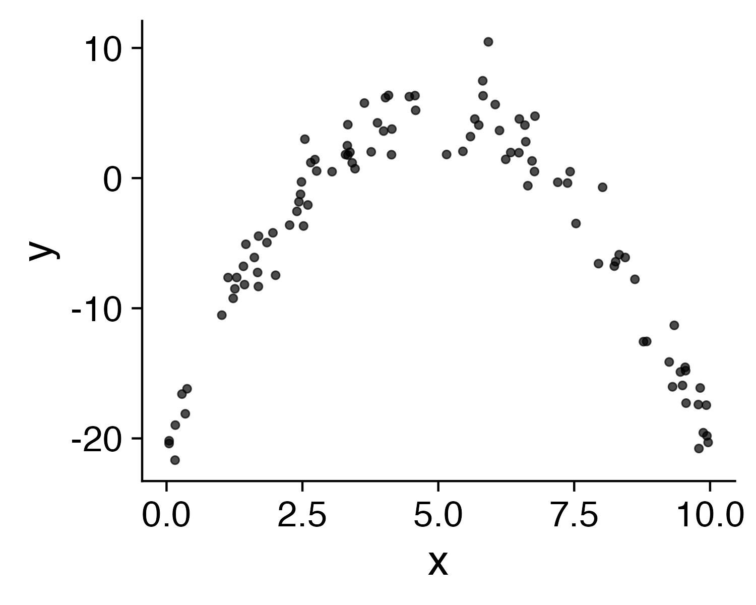
How do you interpret \(r\)?
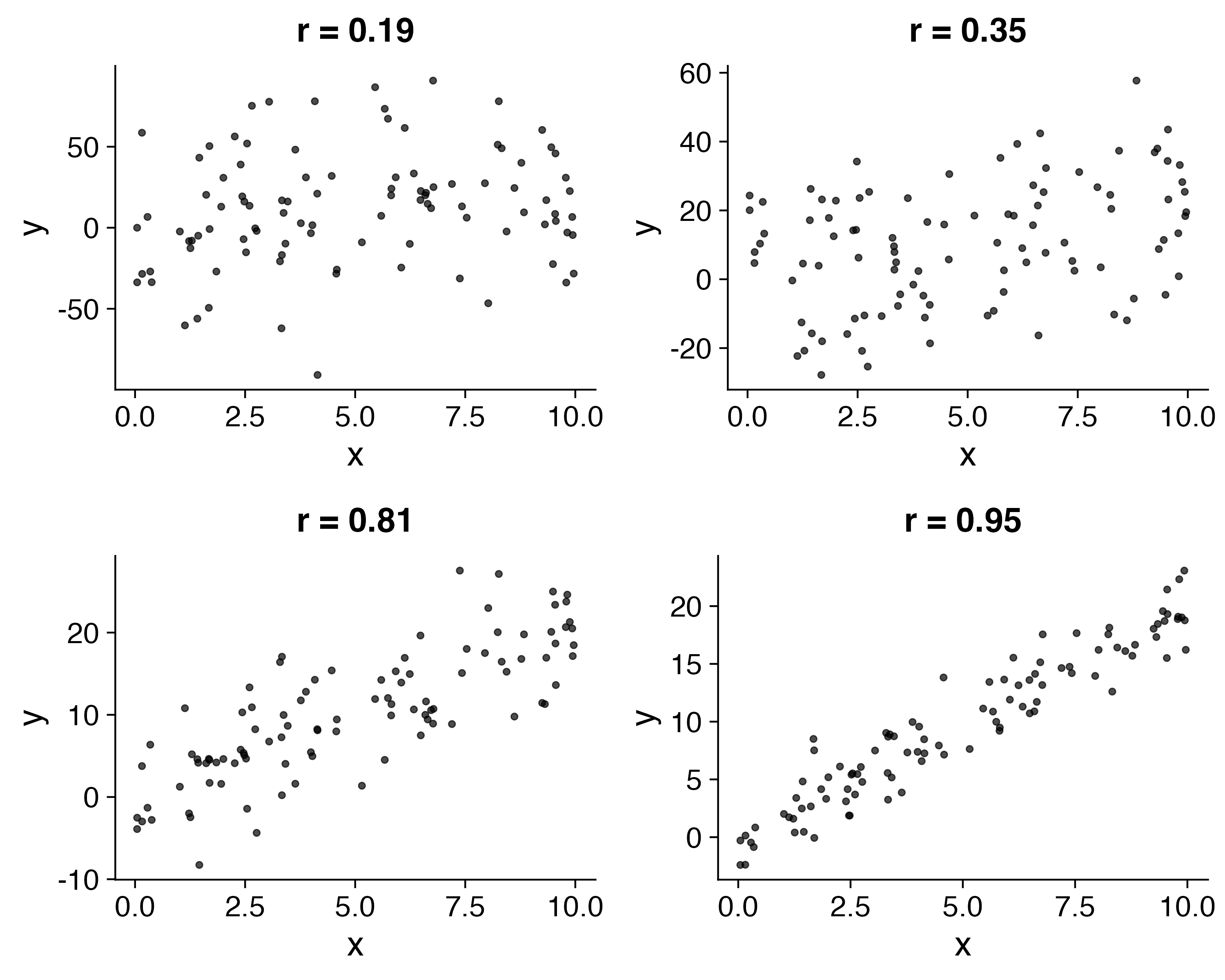
What does \(r\) mean?
- \(\pm 0.1 - 0.3\): Weak
- \(\pm 0.3 - 0.5\): Moderate
- \(\pm 0.5 - 0.8\): Strong
- \(\pm 0.8 - 1.0\): Very strong
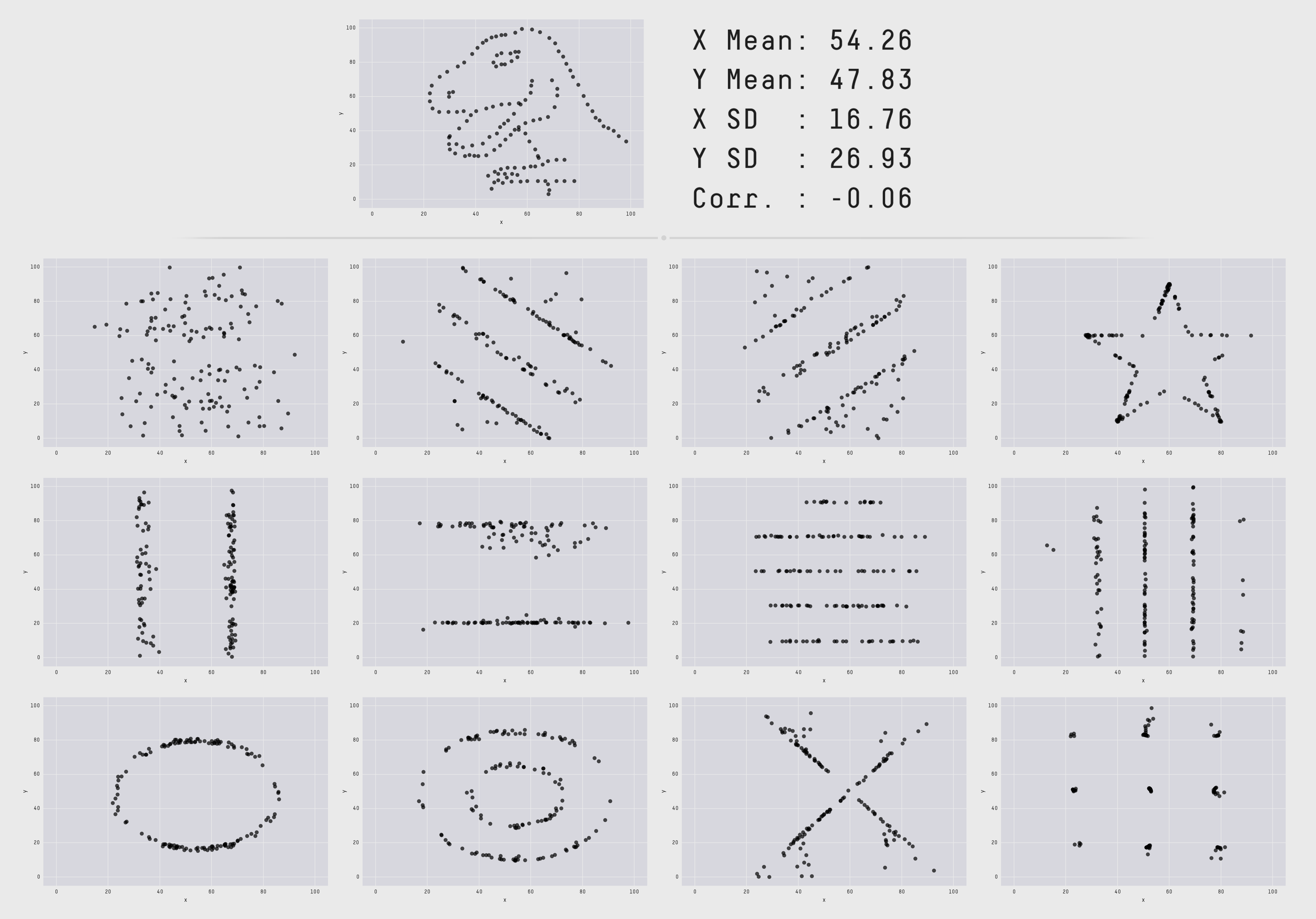
The datasaurus
(More here)
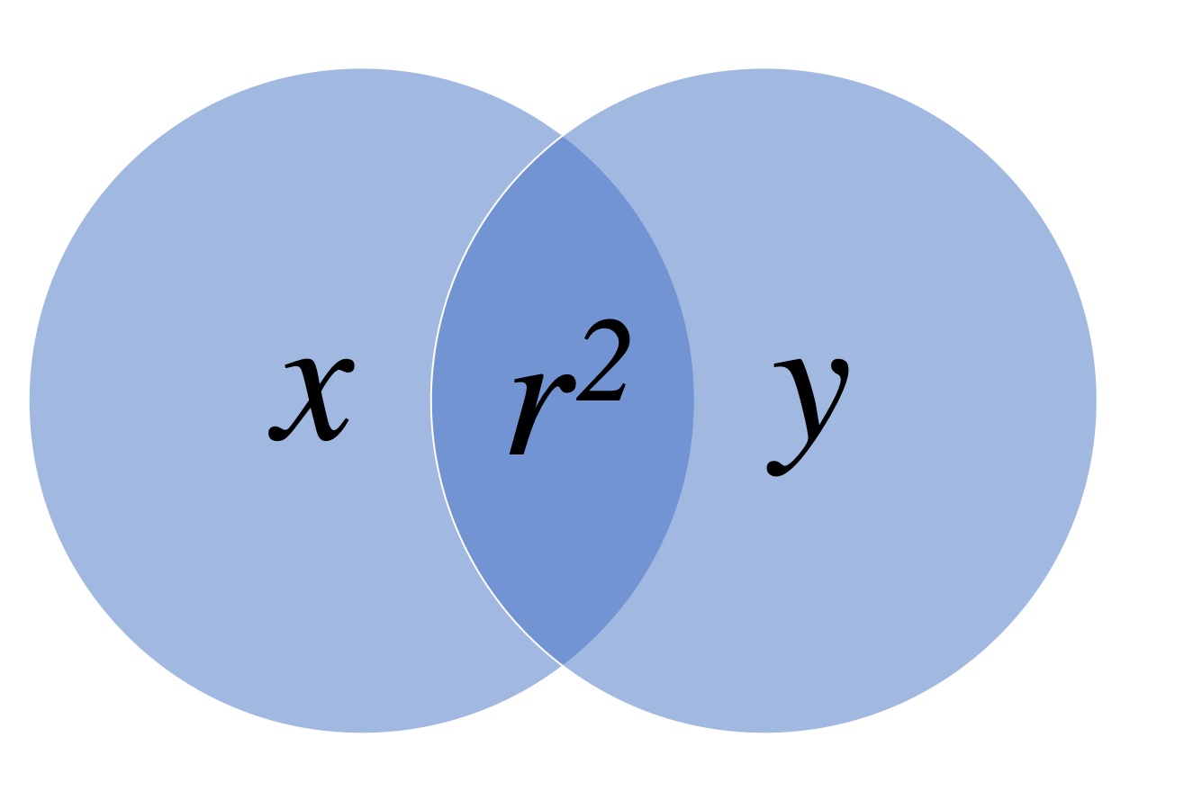
Coefficient of determination: \(r^2\)
Percent of variance in one variable that is explained by the other variable
| \(r\) | \(r^2\) |
|---|---|
| 0.1 | 0.01 |
| 0.2 | 0.04 |
| 0.3 | 0.09 |
| 0.4 | 0.16 |
| 0.5 | 0.25 |
| 0.6 | 0.36 |
| 0.7 | 0.49 |
| 0.8 | 0.64 |
| 0.9 | 0.81 |
| 1.0 | 1.00 |
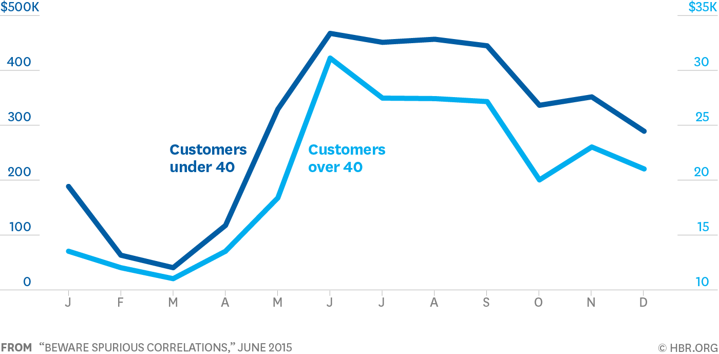
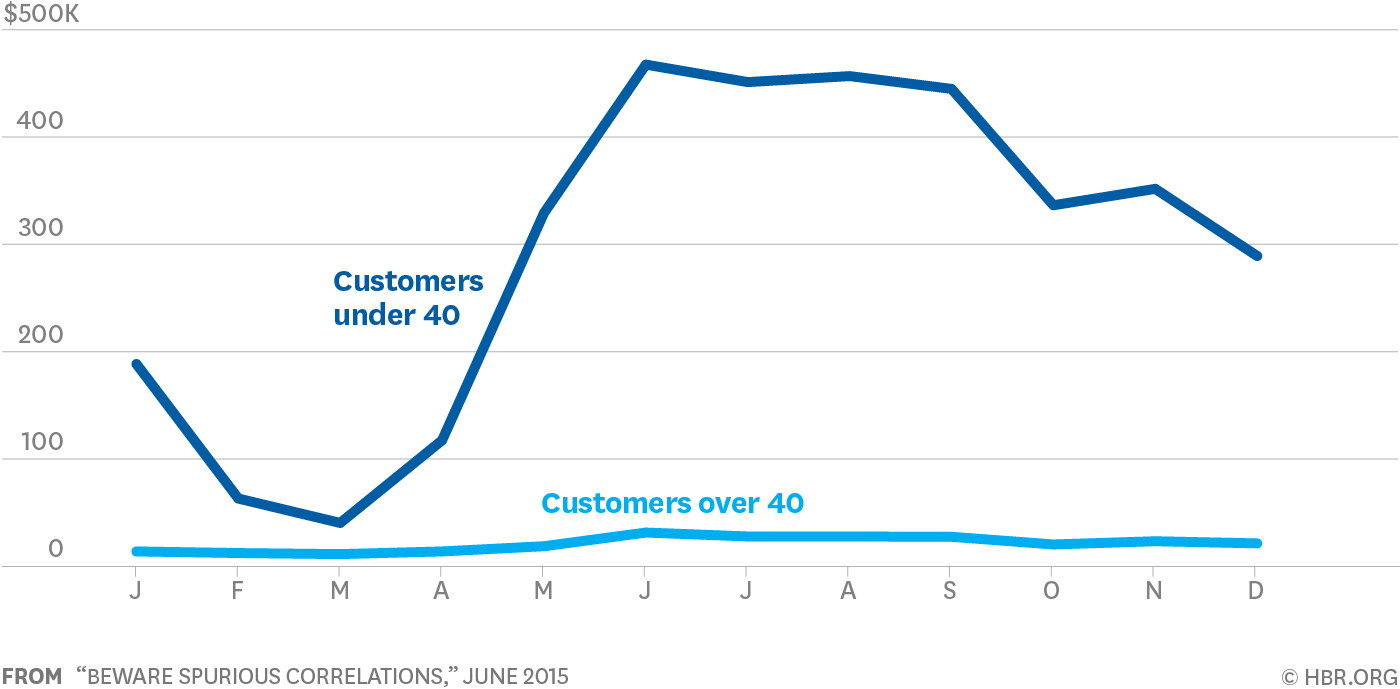
Be weary of dual axes!
(They can cause spurious correlations)
Dual axes
Single axis
Outliers
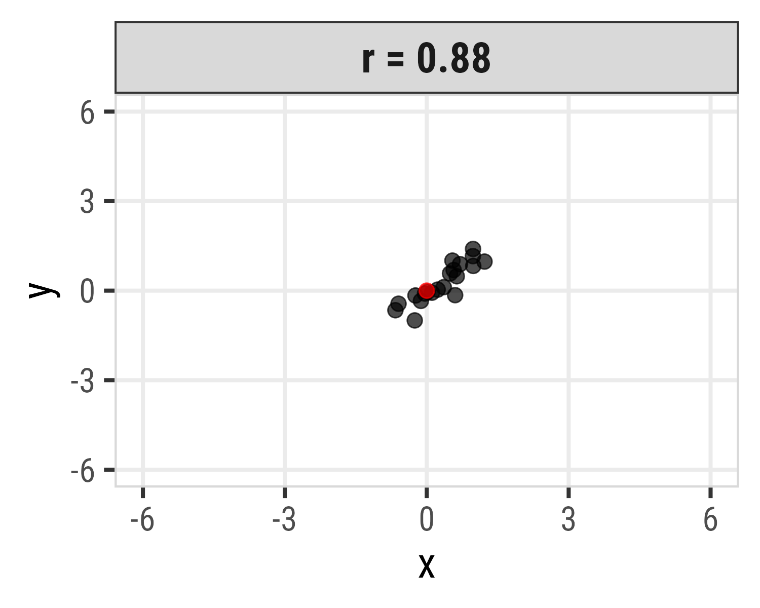
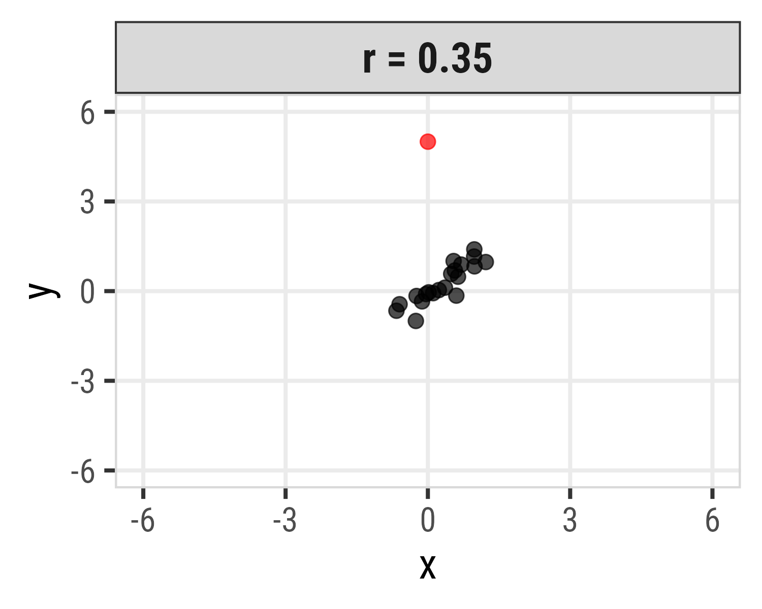
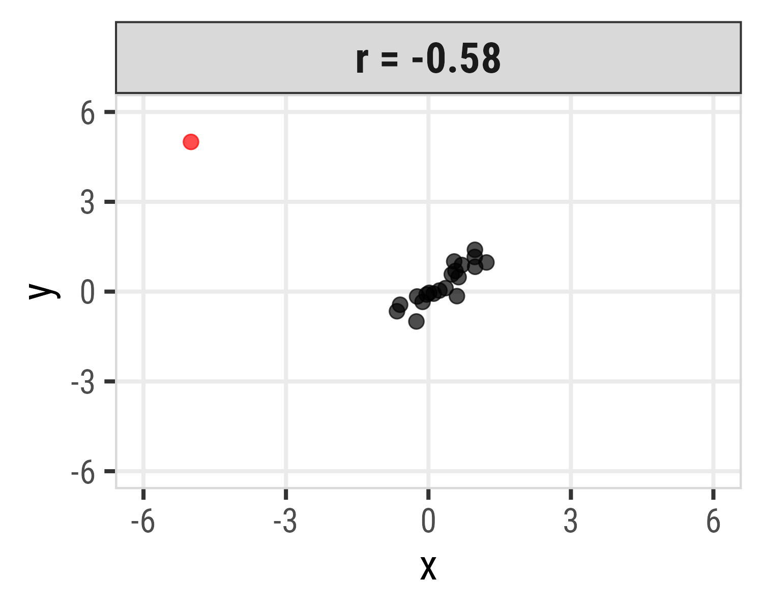
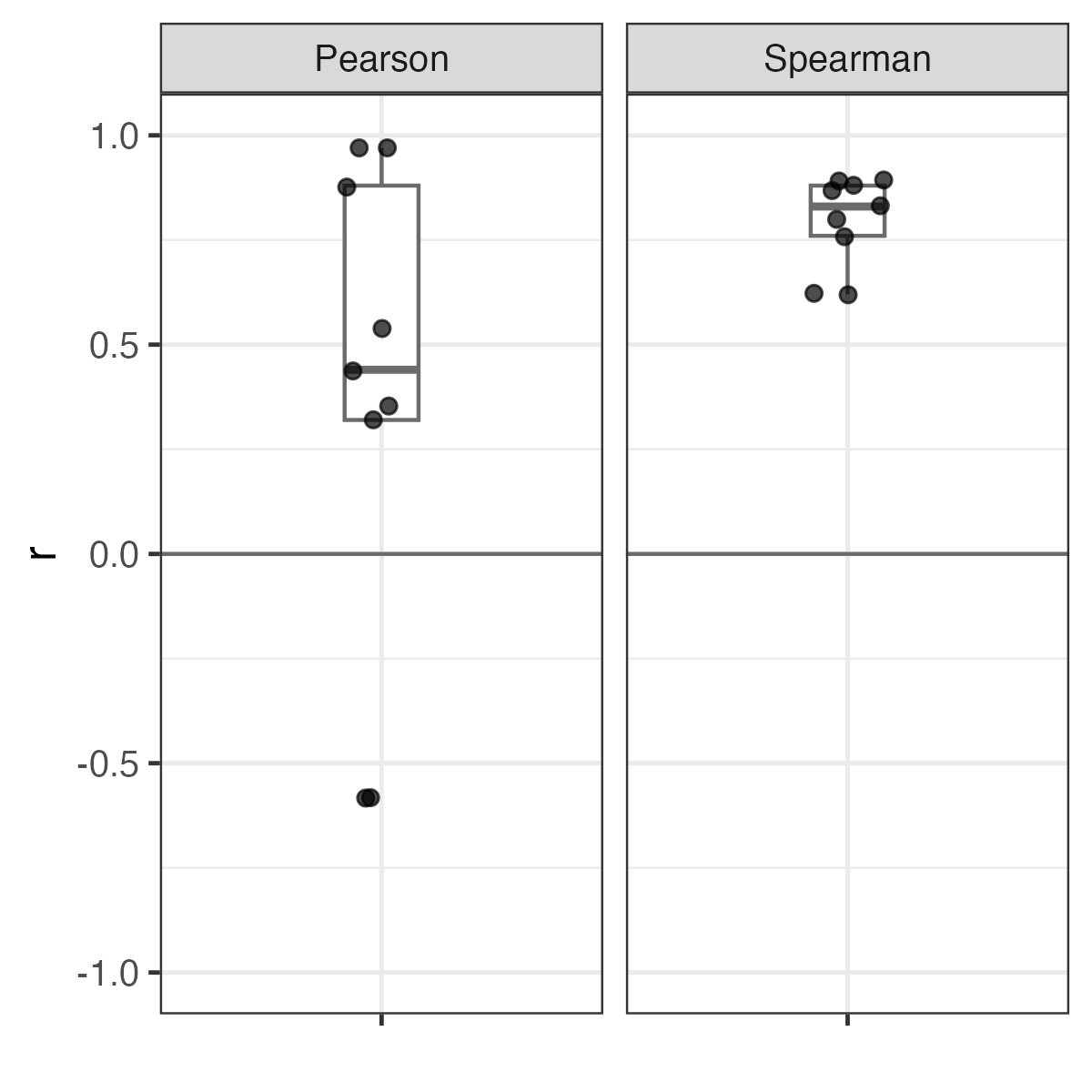
Pearson correlation is highly sensitive to outliers
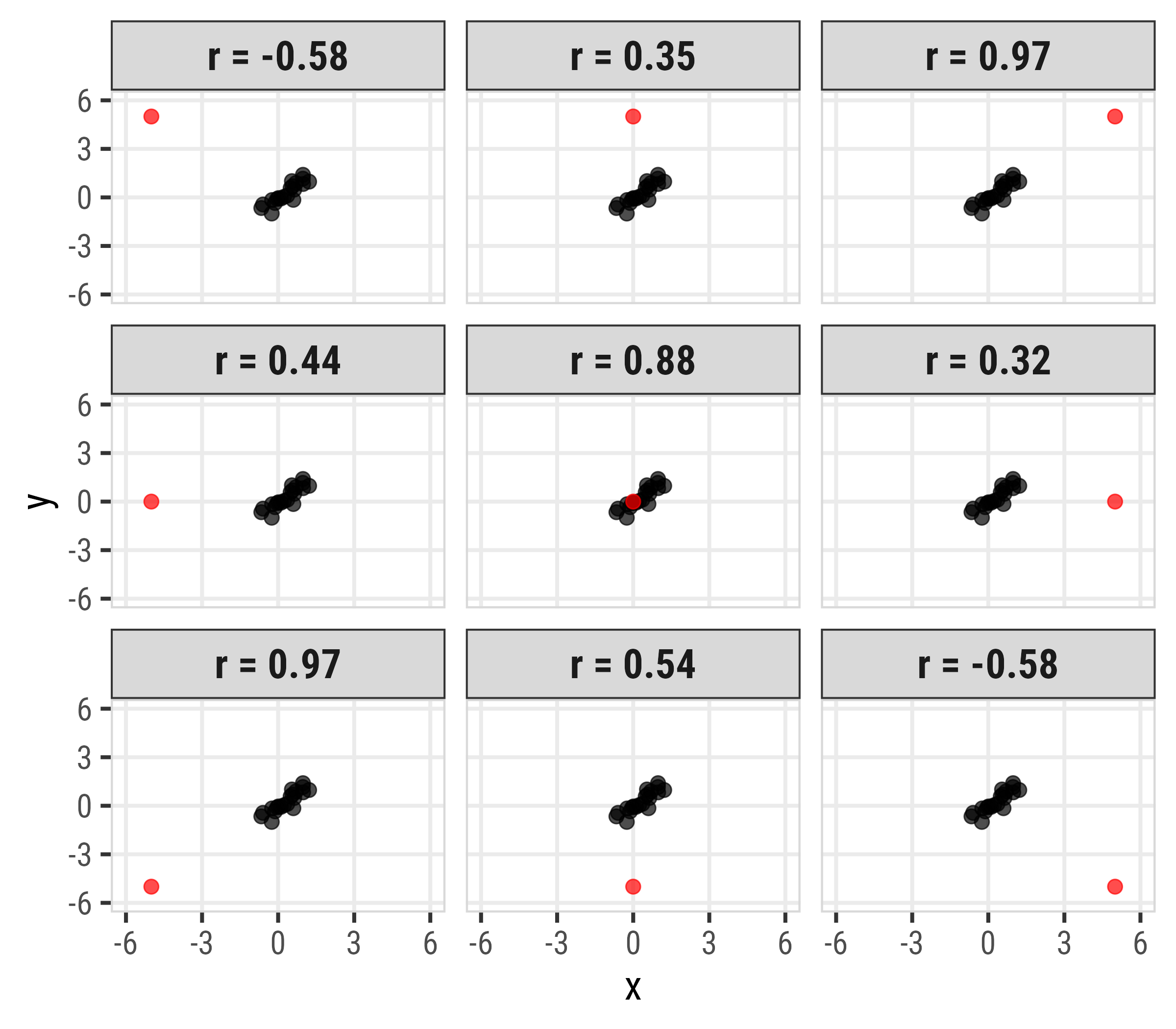
Spearman correlation more robust to outliers
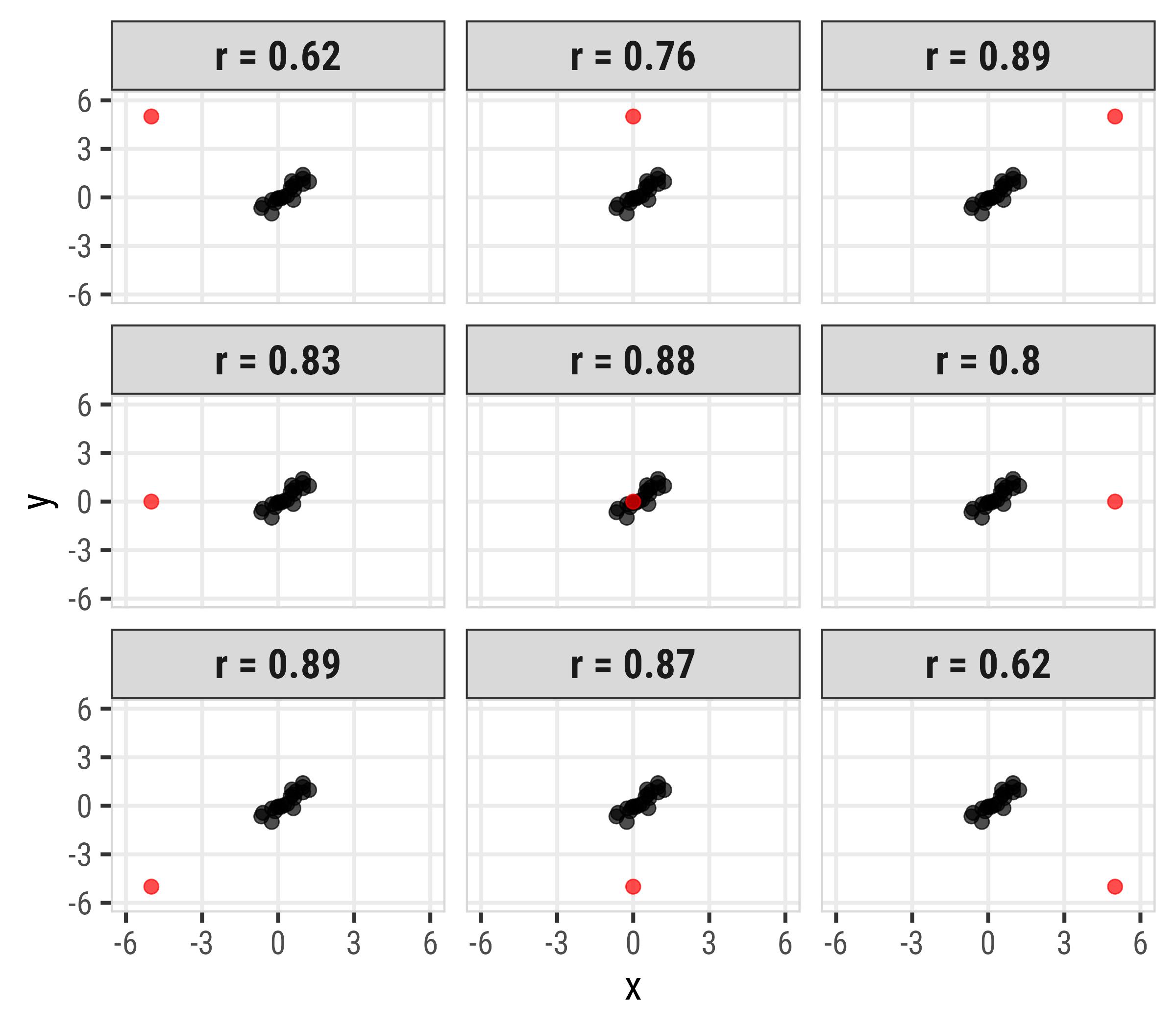
Spearman correlation more robust to outliers
| Pearson | Spearman |
|---|---|
| -0.56 | 0.53 |
| 0.39 | 0.69 |
| 0.94 | 0.81 |
| 0.38 | 0.76 |
| 0.81 | 0.79 |
| 0.31 | 0.70 |
| 0.95 | 0.81 |
| 0.51 | 0.75 |
| -0.56 | 0.53 |
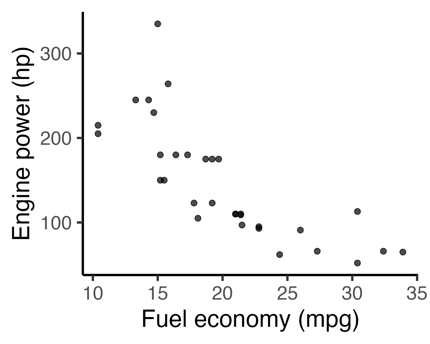
Scatterplots: The correlation workhorse
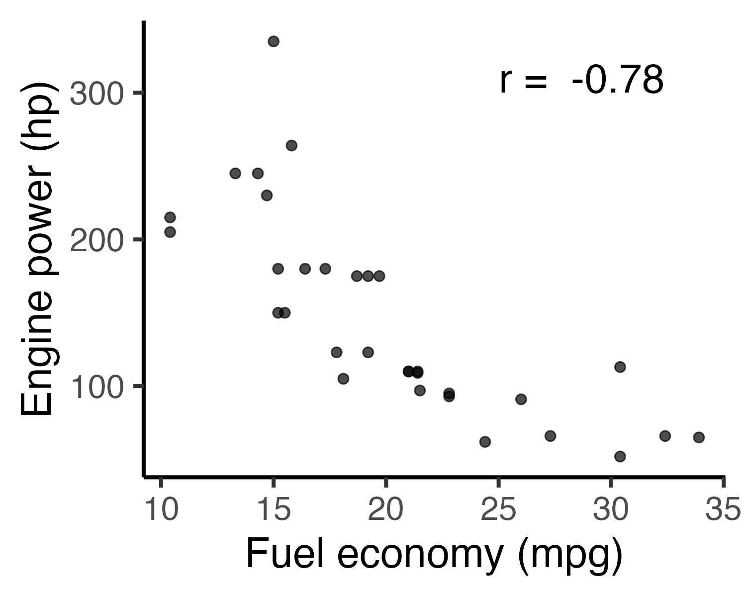
Adding a correlation label to a chart
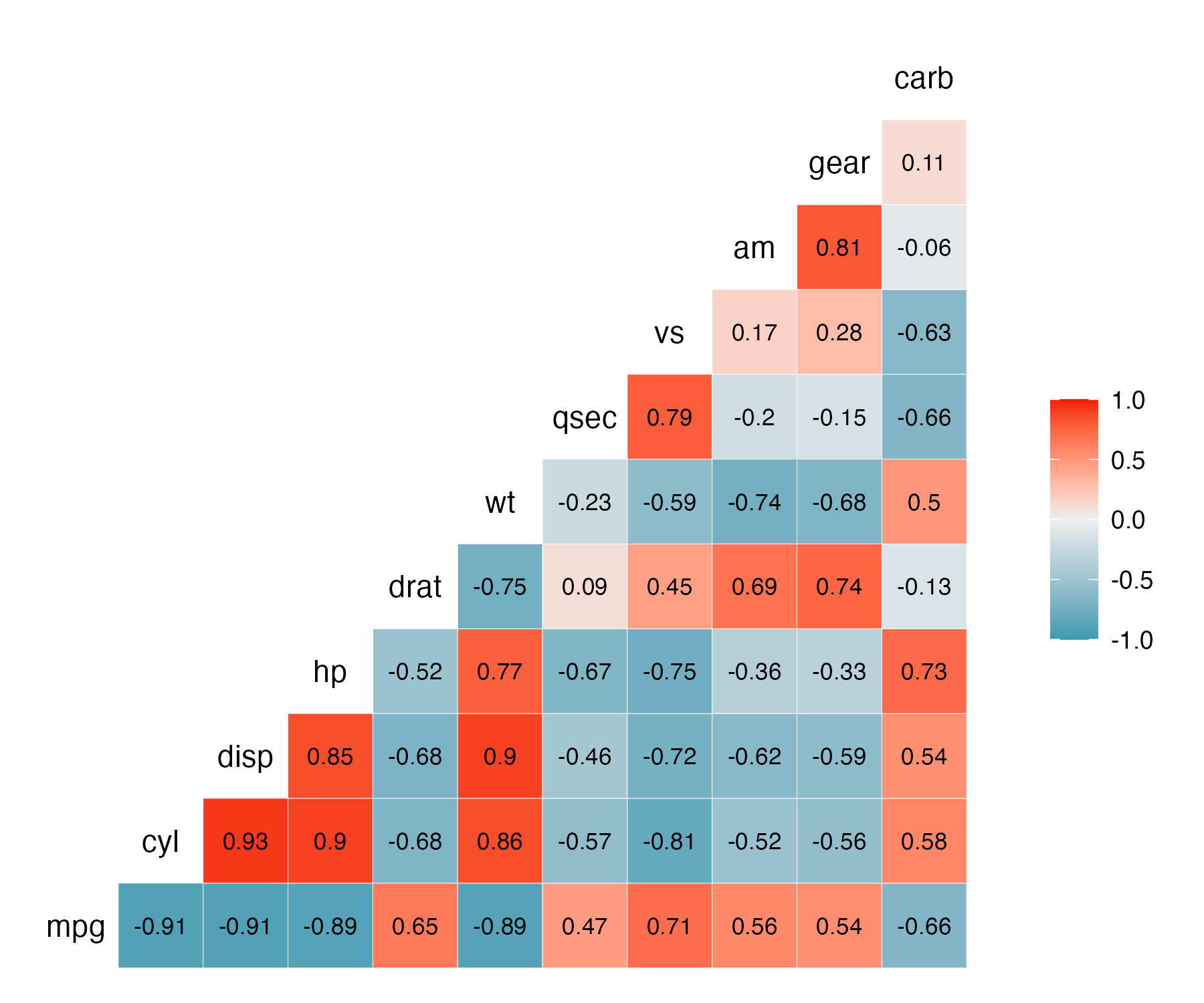
Visualize all the correlations: ggcorr()
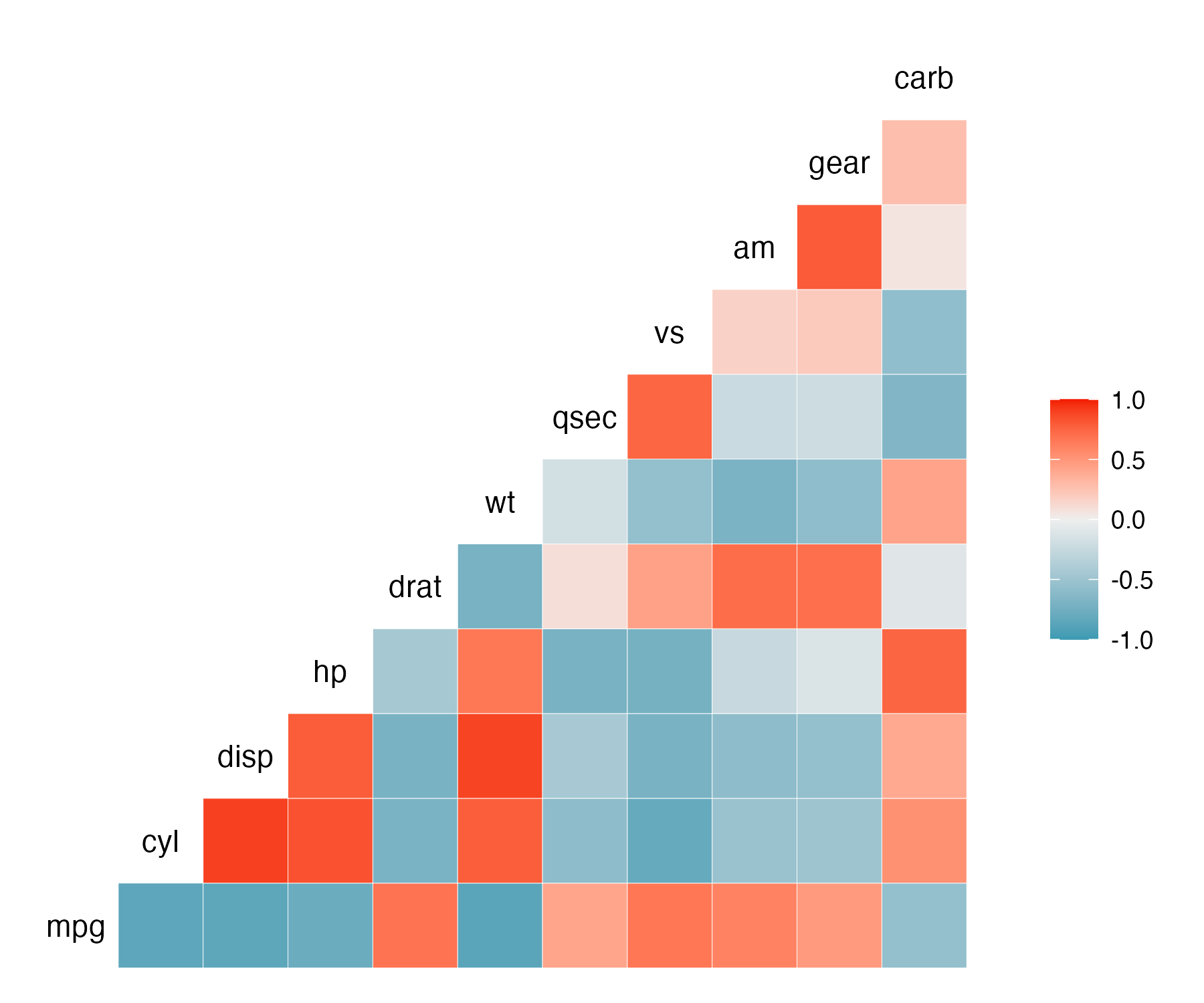
Visualizing correlations: ggcorr()
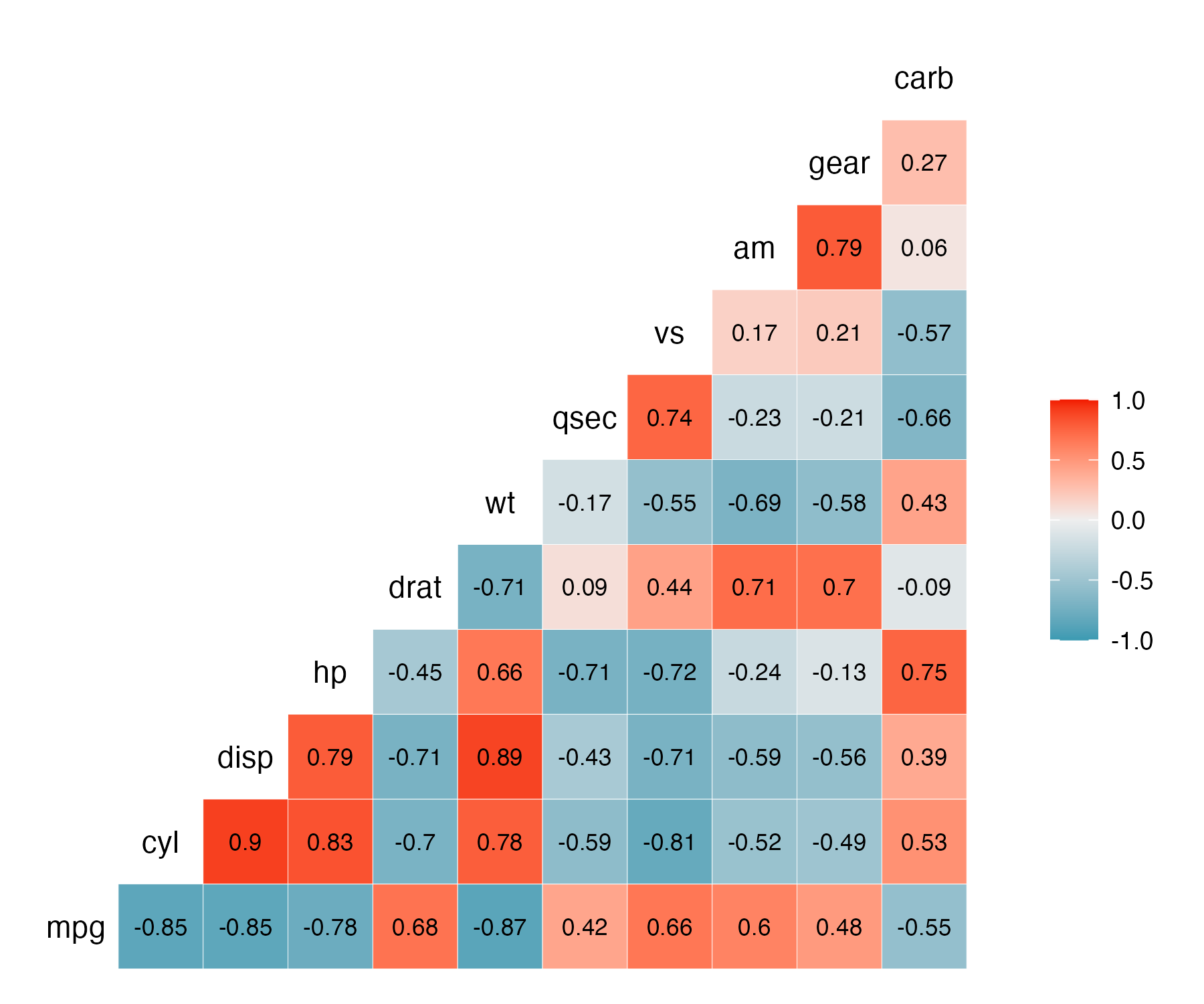
Visualizing correlations: ggcorr()
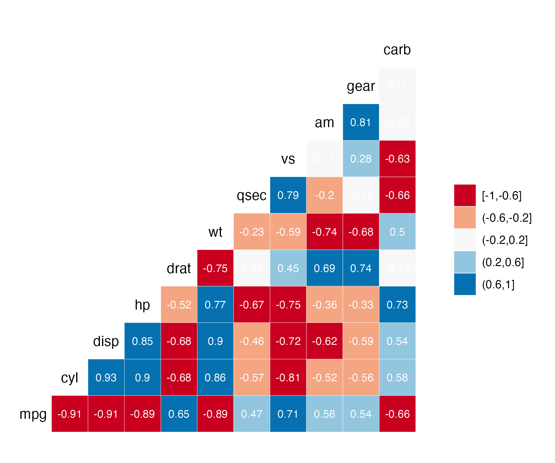
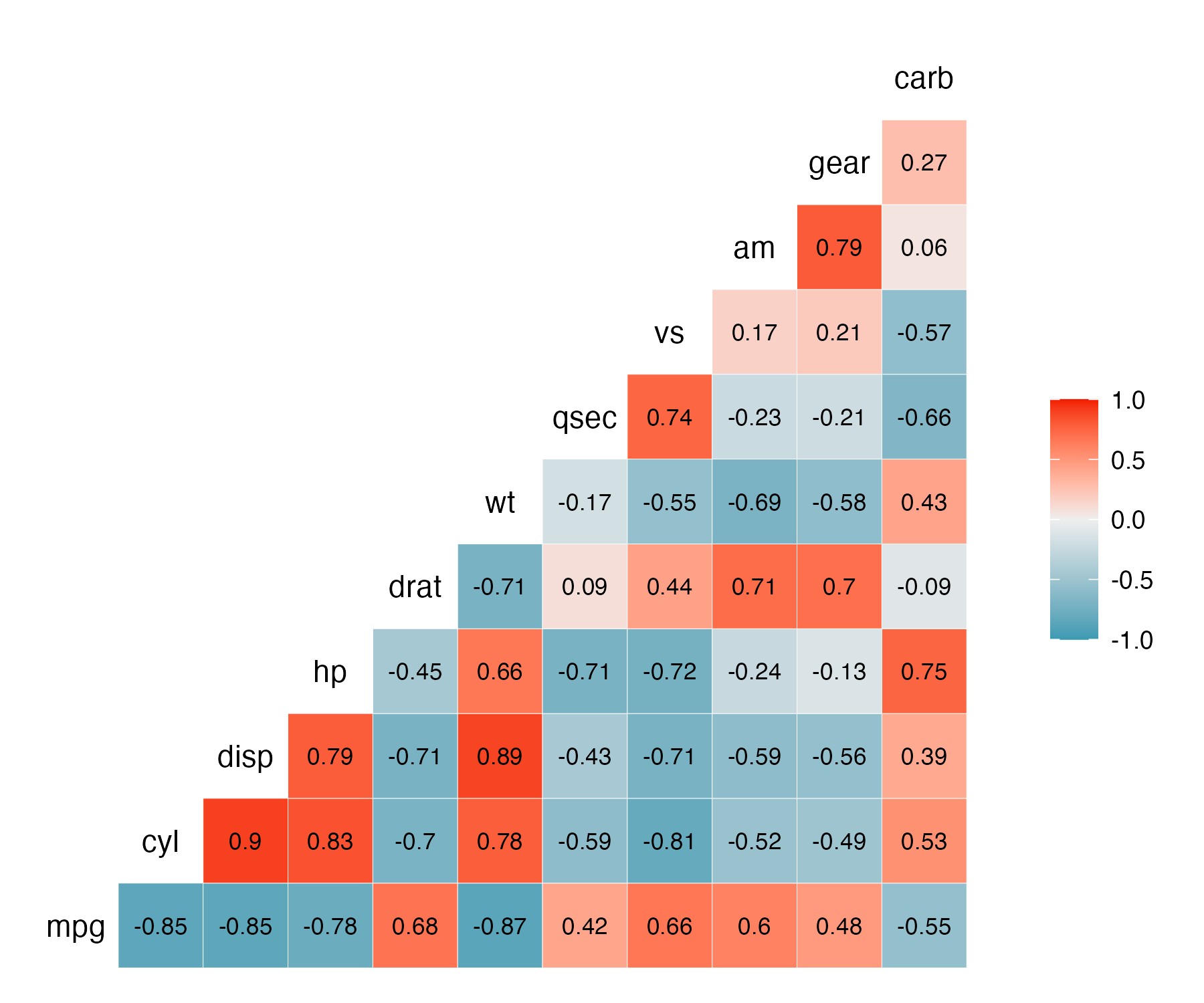
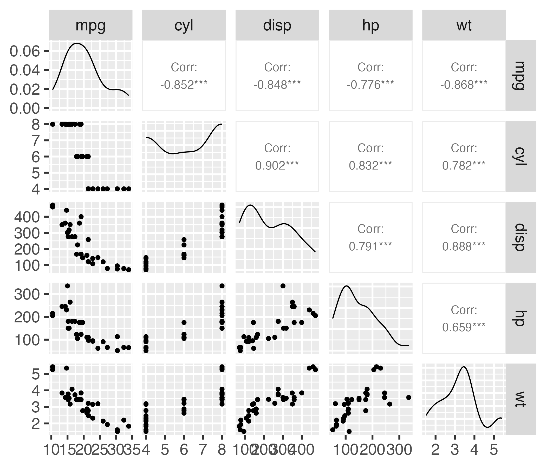
Correlograms: ggpairs()
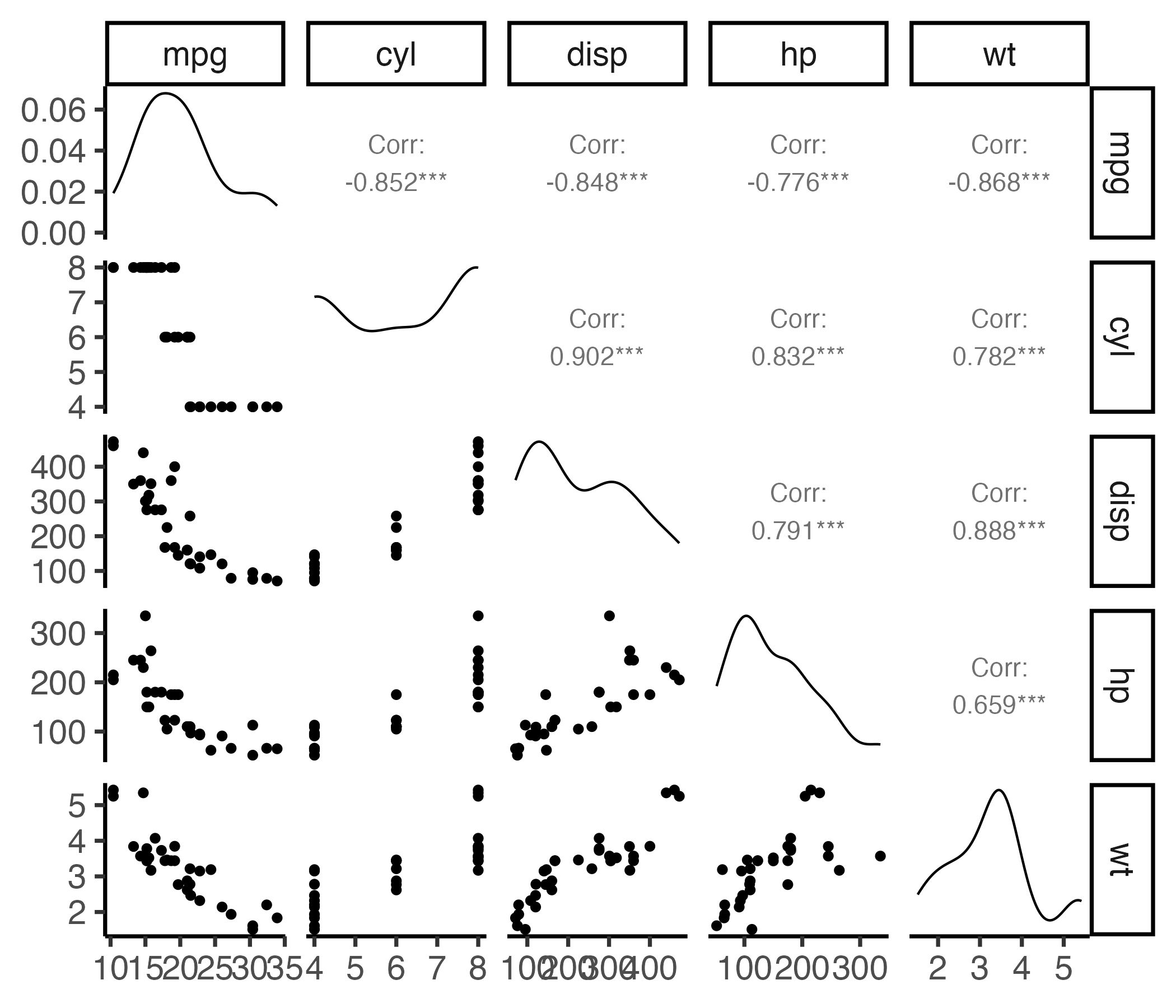
Correlograms: ggpairs()
Your turn
15:00
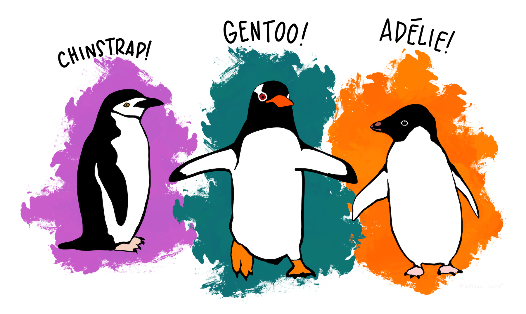
Using the penguins data frame:
Find the two variables with the largest correlation in absolute value (i.e. closest to -1 or 1).
Create a scatter plot of those two variables.
Add an annotation for the Pearson correlation coefficient.
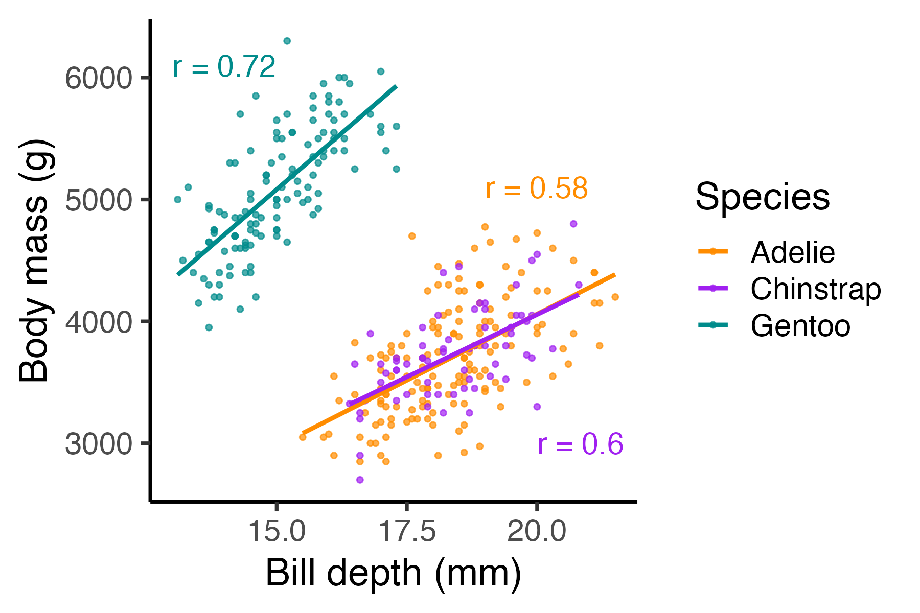
Simpson’s Paradox: when correlation betrays you
Body mass vs. Bill depth
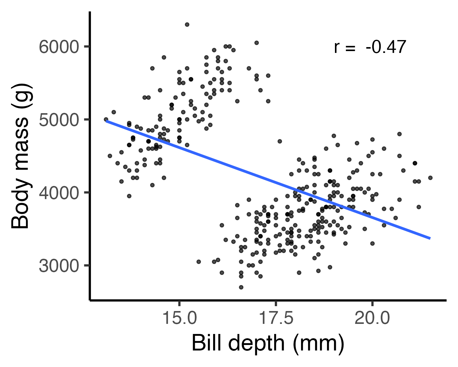
Body mass vs. Bill depth
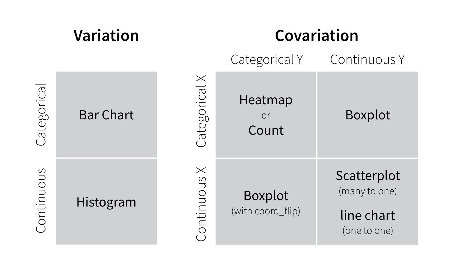
Visualizing variation
Ask yourself:
- What type of variation occurs within my variables?
- What type of covariation occurs between my variables?
Check out these guides
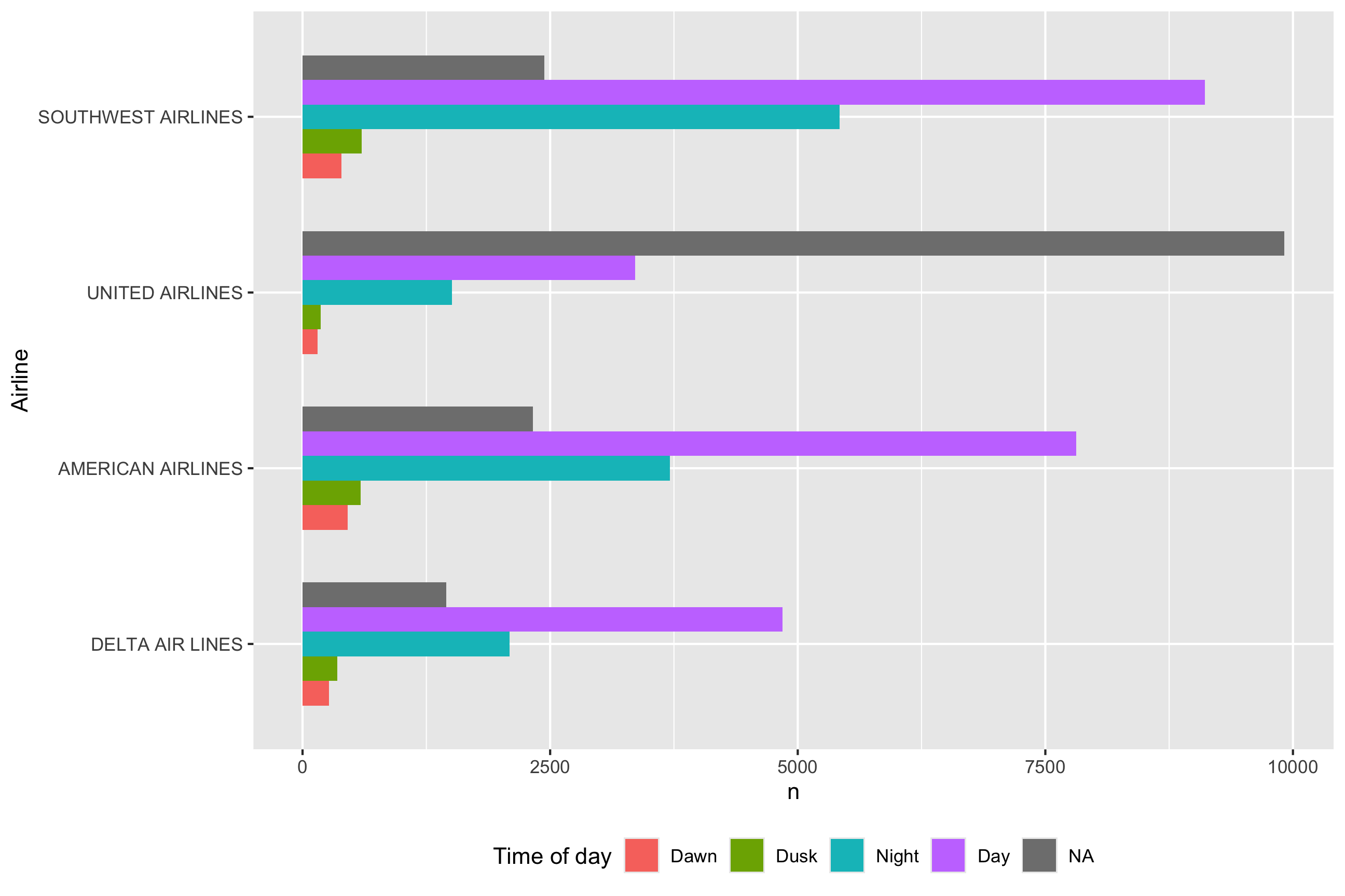
Two Categorical Variables
Visualize with bars:
map fill to denote 2nd categorical var
Two Continuous Variables
Visualize with scatterplot - looking for clustering and/or correlational relationship
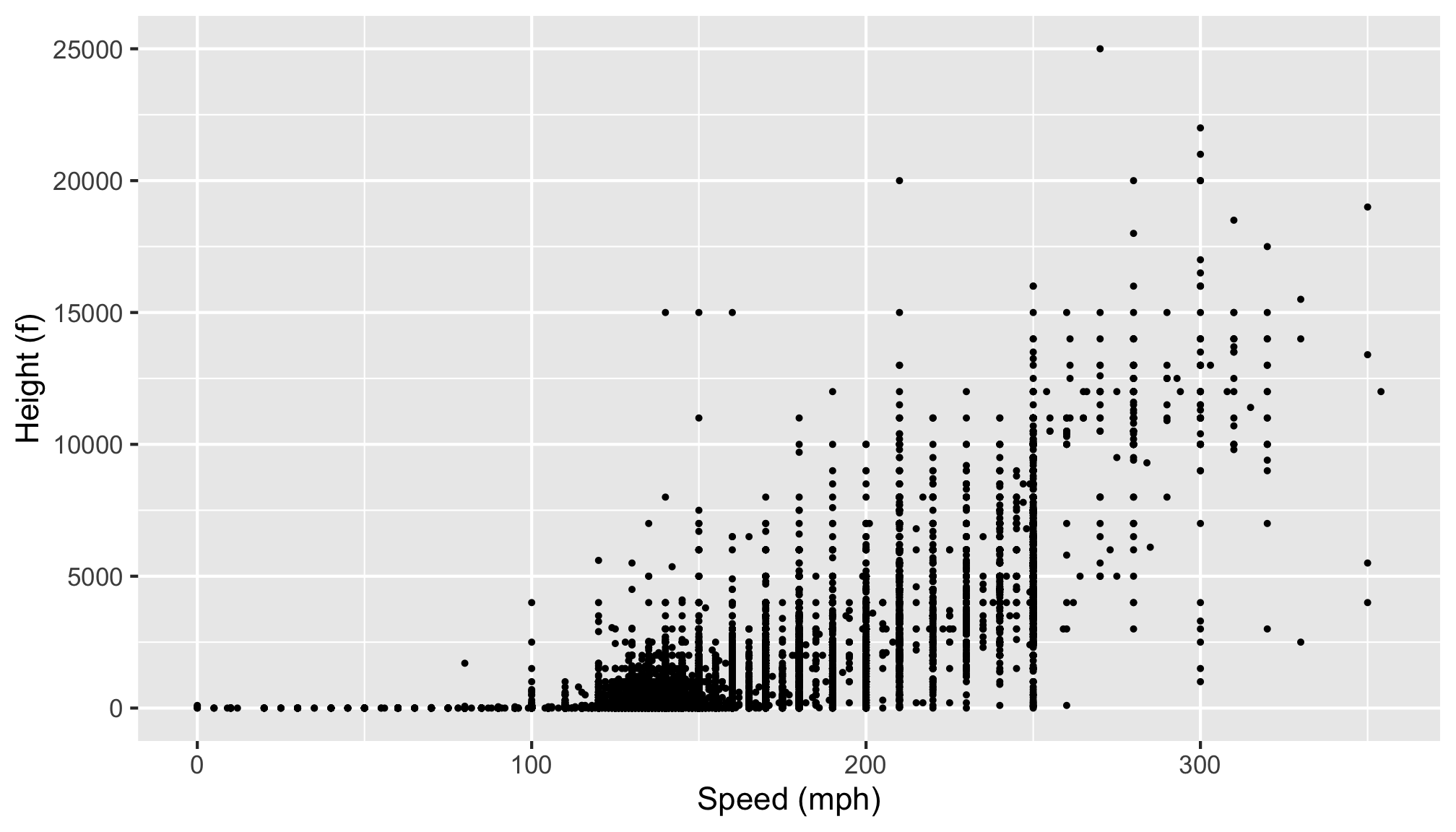
One Continuous, One Categorical
Visualize with boxplot